import geopandas as gpd
import pandas as pd
import altair as alt
geo_states = gpd.read_file('data/gz_2010_us_040_00_500k.json')
df_polls = pd.read_csv('data/presidential_poll_averages_2020.csv')Lab: Choropleth Maps
1 Lab: Choropleth Maps
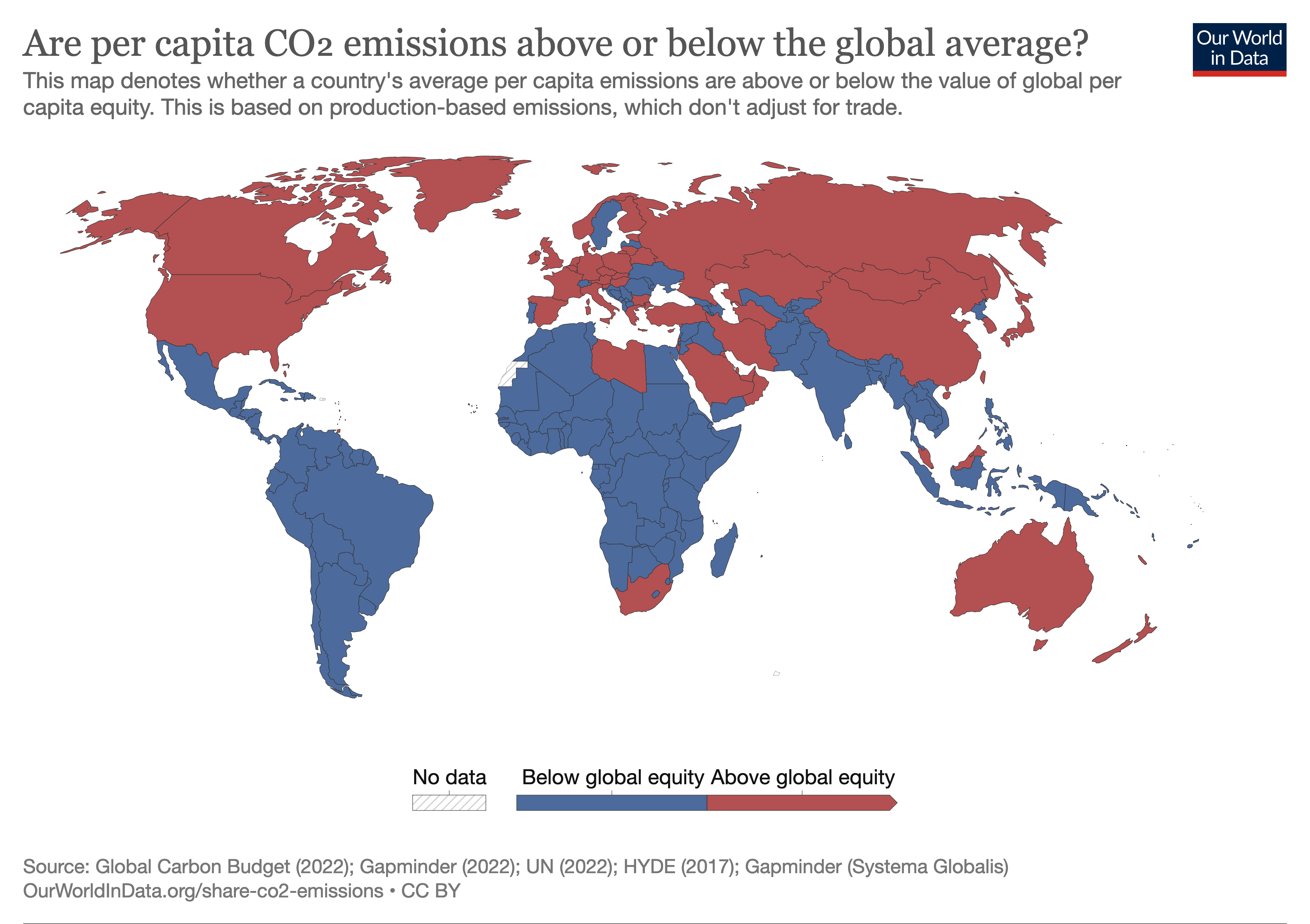
A visualisation often shown is a choropleth. This is a series of spatial polygons (such as states in the USA) which are coloured by a feature, like the one below.
In this lab, we will look at creating choropleths of polling data in the recent USA election, and how maps can sometimes be deceptive (as well as how to detect -and avoid- such techniques). To do so, we will be using geopandas for the geospatial features, and altair for the maps’ visualisations.
About geopandas
geopandas is a very specific and complex library that is not installed by default in Anaconda, so normally you would need to install it (and its multiple dependencies) by yourselves. If you are using the course’s virtual environment, this should be installed for you the first time you set up your environment for the module. Refer to sec-setup for instructions on how to set up your environment.
1.1 Data preparations
We will be loading two datasets:
geo_states: contains the geospatial polygons of the states in America, but does not contain any data about USA elections;df_polls: the polling data we used in the last notebook, but does not have any geospatial polygons (you can find more information about every variable here).
In [1]:
Let’s explore the data first:
In [2]:
geo_states.head()| GEO_ID | STATE | NAME | LSAD | CENSUSAREA | geometry | |
|---|---|---|---|---|---|---|
| 0 | 0400000US23 | 23 | Maine | 30842.923 | MULTIPOLYGON (((-67.61976 44.51975, -67.61541 ... | |
| 1 | 0400000US25 | 25 | Massachusetts | 7800.058 | MULTIPOLYGON (((-70.83204 41.60650, -70.82373 ... | |
| 2 | 0400000US26 | 26 | Michigan | 56538.901 | MULTIPOLYGON (((-88.68443 48.11579, -88.67563 ... | |
| 3 | 0400000US30 | 30 | Montana | 145545.801 | POLYGON ((-104.05770 44.99743, -104.25015 44.9... | |
| 4 | 0400000US32 | 32 | Nevada | 109781.180 | POLYGON ((-114.05060 37.00040, -114.04999 36.9... |
This seems like a regular data frame, but there’s a feature that stands out from the others: geometry. This feature contains the coordinates thar define the polygons (or multipolygons) for every region in the map, in this case, every State in the USA. This is also an indicator that we are not using a regular dataframe, but a particular type of dataframe called GeoDataFrame:
In [3]:
type(geo_states)geopandas.geodataframe.GeoDataFrameBecause this is a geospatial dataframe, we can visualise it as a map. In this case, we are going to use Altair to create a map using the AlbersUsa projection.
In [4]:
alt.Chart(geo_states, title='US states').mark_geoshape().encode(
).properties(
width=500,
height=300
).project(
type='albersUsa'
)And now the polls’ result:
In [5]:
df_polls| cycle | state | modeldate | candidate_name | pct_estimate | pct_trend_adjusted | |
|---|---|---|---|---|---|---|
| 0 | 2020 | Wyoming | 11/3/2020 | Joseph R. Biden Jr. | 30.81486 | 30.82599 |
| 1 | 2020 | Wisconsin | 11/3/2020 | Joseph R. Biden Jr. | 52.12642 | 52.09584 |
| 2 | 2020 | West Virginia | 11/3/2020 | Joseph R. Biden Jr. | 33.49125 | 33.51517 |
| 3 | 2020 | Washington | 11/3/2020 | Joseph R. Biden Jr. | 59.34201 | 59.39408 |
| 4 | 2020 | Virginia | 11/3/2020 | Joseph R. Biden Jr. | 53.74120 | 53.72101 |
| ... | ... | ... | ... | ... | ... | ... |
| 29080 | 2020 | Connecticut | 2/27/2020 | Donald Trump | 33.66370 | 34.58325 |
| 29081 | 2020 | Colorado | 2/27/2020 | Donald Trump | 44.27899 | 44.07662 |
| 29082 | 2020 | California | 2/27/2020 | Donald Trump | 34.66504 | 34.69761 |
| 29083 | 2020 | Arizona | 2/27/2020 | Donald Trump | 47.79450 | 48.07208 |
| 29084 | 2020 | Alabama | 2/27/2020 | Donald Trump | 59.15000 | 59.14228 |
29085 rows × 6 columns
As you can see, modeldate has different dates. Let’s double check that:
In [6]:
df_polls.modeldate.unique()array(['11/3/2020', '11/2/2020', '11/1/2020', '10/31/2020', '10/30/2020',
'10/29/2020', '10/28/2020', '10/27/2020', '10/26/2020',
'10/25/2020', '10/24/2020', '10/23/2020', '10/22/2020',
'10/21/2020', '10/20/2020', '10/19/2020', '10/18/2020',
'10/17/2020', '10/16/2020', '10/15/2020', '10/14/2020',
'10/13/2020', '10/12/2020', '10/11/2020', '10/10/2020',
'10/9/2020', '10/8/2020', '10/7/2020', '10/6/2020', '10/5/2020',
'10/4/2020', '10/3/2020', '10/2/2020', '10/1/2020', '9/30/2020',
'9/29/2020', '9/28/2020', '9/27/2020', '9/26/2020', '9/25/2020',
'9/24/2020', '9/23/2020', '9/22/2020', '9/21/2020', '9/20/2020',
'9/19/2020', '9/18/2020', '9/17/2020', '9/16/2020', '9/15/2020',
'9/14/2020', '9/13/2020', '9/12/2020', '9/11/2020', '9/10/2020',
'9/9/2020', '9/8/2020', '9/7/2020', '9/6/2020', '9/5/2020',
'9/4/2020', '9/3/2020', '9/2/2020', '9/1/2020', '8/31/2020',
'8/30/2020', '8/29/2020', '8/28/2020', '8/27/2020', '8/26/2020',
'8/25/2020', '8/24/2020', '8/23/2020', '8/22/2020', '8/21/2020',
'8/20/2020', '8/19/2020', '8/18/2020', '8/17/2020', '8/16/2020',
'8/15/2020', '8/14/2020', '8/13/2020', '8/12/2020', '8/11/2020',
'8/10/2020', '8/9/2020', '8/8/2020', '8/7/2020', '8/6/2020',
'8/5/2020', '8/4/2020', '8/3/2020', '8/2/2020', '8/1/2020',
'7/31/2020', '7/30/2020', '7/29/2020', '7/28/2020', '7/27/2020',
'7/26/2020', '7/25/2020', '7/24/2020', '7/23/2020', '7/22/2020',
'7/21/2020', '7/20/2020', '7/19/2020', '7/18/2020', '7/17/2020',
'7/16/2020', '7/15/2020', '7/14/2020', '7/13/2020', '7/12/2020',
'7/11/2020', '7/10/2020', '7/9/2020', '7/8/2020', '7/7/2020',
'7/6/2020', '7/5/2020', '7/4/2020', '7/3/2020', '7/2/2020',
'7/1/2020', '6/30/2020', '6/29/2020', '6/28/2020', '6/27/2020',
'6/26/2020', '6/25/2020', '6/24/2020', '6/23/2020', '6/22/2020',
'6/21/2020', '6/20/2020', '6/19/2020', '6/18/2020', '6/17/2020',
'6/16/2020', '6/15/2020', '6/14/2020', '6/13/2020', '6/12/2020',
'6/11/2020', '6/10/2020', '6/9/2020', '6/8/2020', '6/7/2020',
'6/6/2020', '6/5/2020', '6/4/2020', '6/3/2020', '6/2/2020',
'6/1/2020', '5/31/2020', '5/30/2020', '5/29/2020', '5/28/2020',
'5/27/2020', '5/26/2020', '5/25/2020', '5/24/2020', '5/23/2020',
'5/22/2020', '5/21/2020', '5/20/2020', '5/19/2020', '5/18/2020',
'5/17/2020', '5/16/2020', '5/15/2020', '5/14/2020', '5/13/2020',
'5/12/2020', '5/11/2020', '5/10/2020', '5/9/2020', '5/8/2020',
'5/7/2020', '5/6/2020', '5/5/2020', '5/4/2020', '5/3/2020',
'5/2/2020', '5/1/2020', '4/30/2020', '4/29/2020', '4/28/2020',
'4/27/2020', '4/26/2020', '4/25/2020', '4/24/2020', '4/23/2020',
'4/22/2020', '4/21/2020', '4/20/2020', '4/19/2020', '4/18/2020',
'4/17/2020', '4/16/2020', '4/15/2020', '4/14/2020', '4/13/2020',
'4/12/2020', '4/11/2020', '4/10/2020', '4/9/2020', '4/8/2020',
'4/7/2020', '4/6/2020', '4/5/2020', '4/4/2020', '4/3/2020',
'4/2/2020', '4/1/2020', '3/31/2020', '3/30/2020', '3/29/2020',
'3/28/2020', '3/27/2020', '3/26/2020', '3/25/2020', '3/24/2020',
'3/23/2020', '3/22/2020', '3/21/2020', '3/20/2020', '3/19/2020',
'3/18/2020', '3/17/2020', '3/16/2020', '3/15/2020', '3/14/2020',
'3/13/2020', '3/12/2020', '3/11/2020', '3/10/2020', '3/9/2020',
'3/8/2020', '3/7/2020', '3/6/2020', '3/5/2020', '3/4/2020',
'3/3/2020', '3/2/2020', '3/1/2020', '2/29/2020', '2/28/2020',
'2/27/2020'], dtype=object)1.1.1 Filtering
That means, that we will need to filter our poll data to a specific date, in this case 11/2/2020
In [7]:
df_nov = df_polls[
(df_polls.modeldate == '11/3/2020')
]
df_nov_states = df_nov[
(df_nov.candidate_name == 'Donald Trump') |
(df_nov.candidate_name == 'Joseph R. Biden Jr.')
]
df_nov_states| cycle | state | modeldate | candidate_name | pct_estimate | pct_trend_adjusted | |
|---|---|---|---|---|---|---|
| 0 | 2020 | Wyoming | 11/3/2020 | Joseph R. Biden Jr. | 30.81486 | 30.82599 |
| 1 | 2020 | Wisconsin | 11/3/2020 | Joseph R. Biden Jr. | 52.12642 | 52.09584 |
| 2 | 2020 | West Virginia | 11/3/2020 | Joseph R. Biden Jr. | 33.49125 | 33.51517 |
| 3 | 2020 | Washington | 11/3/2020 | Joseph R. Biden Jr. | 59.34201 | 59.39408 |
| 4 | 2020 | Virginia | 11/3/2020 | Joseph R. Biden Jr. | 53.74120 | 53.72101 |
| ... | ... | ... | ... | ... | ... | ... |
| 107 | 2020 | California | 11/3/2020 | Donald Trump | 32.28521 | 32.43615 |
| 108 | 2020 | Arkansas | 11/3/2020 | Donald Trump | 58.39097 | 58.94886 |
| 109 | 2020 | Arizona | 11/3/2020 | Donald Trump | 46.11074 | 46.10181 |
| 110 | 2020 | Alaska | 11/3/2020 | Donald Trump | 50.99835 | 51.23236 |
| 111 | 2020 | Alabama | 11/3/2020 | Donald Trump | 57.36153 | 57.36126 |
112 rows × 6 columns
1.1.2 Computing percentages
We want to put the percentage estimates for each candidate onto the map. First, let us create a dataframe containing the data for each candidate.
In [8]:
# Create separate data frame for Trump and Biden
trump_data = df_nov_states[
df_nov_states.candidate_name == 'Donald Trump'
]
biden_data = df_nov_states[
df_nov_states.candidate_name == 'Joseph R. Biden Jr.'
]1.1.3 Joining data
As we have seen before, we have two datasets that partially address our needs: geo_states contains the geospatial polygons of the states in America, but lacks data about USA elections; df_polls contains data about USA elections but lacks geometry.
We will need to combine both (joining) to create a (geospatial)dataframe that contains geometry AND polling data so we can create a choropleth map capable of answering our question: who is winning the elections?
To do so, we need to join both dataframes using a common feature. Our spatial and poll data have the name of the state in common, but their columns have different names.
We could rename the columns names, and then join them with pd.merge() but instead, we are going to use a less destructive way.
We can join the geospatial data and poll data using pd.merge() while providing different column names by using left_on for the left data (usually the geodataframe) and right_on for the right dataframe. We will be using this method, as it doesn’t require to rename columns.
In [9]:
# Add the poll data (divided in two data frames) to a single geospatial dataframe.
geo_states_trump = geo_states.merge(
trump_data, left_on = 'NAME', right_on = 'state')
geo_states_biden = geo_states.merge(
biden_data, left_on = 'NAME', right_on = 'state')In [10]:
geo_states_trump.head()| GEO_ID | STATE | NAME | LSAD | CENSUSAREA | geometry | cycle | state | modeldate | candidate_name | pct_estimate | pct_trend_adjusted | |
|---|---|---|---|---|---|---|---|---|---|---|---|---|
| 0 | 0400000US23 | 23 | Maine | 30842.923 | MULTIPOLYGON (((-67.61976 44.51975, -67.61541 ... | 2020 | Maine | 11/3/2020 | Donald Trump | 40.34410 | 40.31588 | |
| 1 | 0400000US25 | 25 | Massachusetts | 7800.058 | MULTIPOLYGON (((-70.83204 41.60650, -70.82373 ... | 2020 | Massachusetts | 11/3/2020 | Donald Trump | 28.56164 | 28.86275 | |
| 2 | 0400000US26 | 26 | Michigan | 56538.901 | MULTIPOLYGON (((-88.68443 48.11579, -88.67563 ... | 2020 | Michigan | 11/3/2020 | Donald Trump | 43.20577 | 43.23326 | |
| 3 | 0400000US30 | 30 | Montana | 145545.801 | POLYGON ((-104.05770 44.99743, -104.25015 44.9... | 2020 | Montana | 11/3/2020 | Donald Trump | 49.74744 | 49.78661 | |
| 4 | 0400000US32 | 32 | Nevada | 109781.180 | POLYGON ((-114.05060 37.00040, -114.04999 36.9... | 2020 | Nevada | 11/3/2020 | Donald Trump | 44.32982 | 44.36094 |
In [11]:
geo_states_biden.head()| GEO_ID | STATE | NAME | LSAD | CENSUSAREA | geometry | cycle | state | modeldate | candidate_name | pct_estimate | pct_trend_adjusted | |
|---|---|---|---|---|---|---|---|---|---|---|---|---|
| 0 | 0400000US23 | 23 | Maine | 30842.923 | MULTIPOLYGON (((-67.61976 44.51975, -67.61541 ... | 2020 | Maine | 11/3/2020 | Joseph R. Biden Jr. | 53.31518 | 53.32106 | |
| 1 | 0400000US25 | 25 | Massachusetts | 7800.058 | MULTIPOLYGON (((-70.83204 41.60650, -70.82373 ... | 2020 | Massachusetts | 11/3/2020 | Joseph R. Biden Jr. | 64.36328 | 64.62505 | |
| 2 | 0400000US26 | 26 | Michigan | 56538.901 | MULTIPOLYGON (((-88.68443 48.11579, -88.67563 ... | 2020 | Michigan | 11/3/2020 | Joseph R. Biden Jr. | 51.17806 | 51.15482 | |
| 3 | 0400000US30 | 30 | Montana | 145545.801 | POLYGON ((-104.05770 44.99743, -104.25015 44.9... | 2020 | Montana | 11/3/2020 | Joseph R. Biden Jr. | 45.34418 | 45.36695 | |
| 4 | 0400000US32 | 32 | Nevada | 109781.180 | POLYGON ((-114.05060 37.00040, -114.04999 36.9... | 2020 | Nevada | 11/3/2020 | Joseph R. Biden Jr. | 49.62386 | 49.65657 |
Joe Biden is clearly winning. Can we make it look like he is not?
1.2 Data visualisation
We can plot this specifying the feature to use for our colour.
In [12]:
alt.Chart(geo_states_trump, title='Poll estimate for Donald Trump on 11/3/2020').mark_geoshape().encode(
color='pct_estimate',
tooltip=['NAME', 'pct_estimate']
).properties(
width=500,
height=300
).project(
type='albersUsa'
)1.2.1 Binning
To smooth out any differences we can bin our data.
In the case below, we will be binning based on a single value (step):
In [13]:
alt.Chart(geo_states_trump, title='Poll estimate for Donald Trump on 11/3/2020').mark_geoshape().encode(
alt.Color('pct_estimate', bin=alt.Bin(step=35)),
tooltip=['NAME', 'pct_estimate']
).properties(
width=500,
height=300
).project(
type='albersUsa'
)
Your turn
How would you interpret the plot above? What would change if we change the value of the step?
What about if we increase the binstep so we have more bins?
In [14]:
alt.Chart(geo_states_trump, title='Poll estimate for Donald Trump on 11/3/2020').mark_geoshape().encode(
alt.Color('pct_estimate', bin=alt.Bin(step=5)),
tooltip=['NAME', 'pct_estimate']
).properties(
width=500,
height=300
).project(
type='albersUsa'
)
Your turn
Try different step sizes for the bins and consider how bins can shape our interpretation of the data. What would happen if plots with different bin sizes were placed side to side?
To add further confusion, what happens when we log scale the data?
In [15]:
alt.Chart(geo_states_trump, title='Poll estimate for Donald Trump on 11/3/2020').mark_geoshape().encode(
alt.Color('pct_estimate', bin=alt.Bin(step=5), scale=alt.Scale(type='log')),
tooltip=['NAME', 'pct_estimate']
).properties(
width=500,
height=300
).project(
type='albersUsa'
)vs
In [16]:
alt.Chart(geo_states_biden, title='Poll estimate for Joe Biden on 11/3/2020').mark_geoshape().encode(
alt.Color('pct_estimate', bin=alt.Bin(step=5), scale=alt.Scale(type='log')),
tooltip=['NAME', 'pct_estimate']
).properties(
width=500,
height=300
).project(
type='albersUsa'
)What is happening here?!?!
1.2.2 Colour palettes
Next up, what about the colours we use and the range of values assigned to each color? Code inspired by/taken from here.
In [17]:
alt.Chart(geo_states_trump, title='Poll estimate for Donal Trump on 11/3/2020').mark_geoshape().encode(
alt.Color('pct_estimate',
scale=alt.Scale(type="linear",
domain=[10, 40, 50, 55, 60, 61, 62],
range=["#414487","#414487",
"#355f8d","#355f8d",
"#2a788e",
"#fde725","#fde725"])),
tooltip=['NAME', 'pct_estimate']
).properties(
width=500,
height=300
).project(
type='albersUsa'
)Compare that with
In [18]:
alt.Chart(geo_states_trump, title='Poll estimate for Donald Trump on 11/3/2020').mark_geoshape().encode(
alt.Color('pct_estimate',
scale=alt.Scale(type="linear",
domain=[10, 20, 30, 35, 68, 70, 100],
range=["#414487","#414487",
"#7ad151","#7ad151",
"#bddf26",
"#fde725","#fde725"])),
tooltip=['NAME', 'pct_estimate']
).properties(
width=500,
height=300
).project(
type='albersUsa'
)1.2.3 Legends
My goodness! So what have we played around with?
- Transforming our scale using log
- Binning our data to smooth out variances
- Altering our colour scheme and the ranges for each colour
… what about if we remove the legend?
In [19]:
alt.Chart(geo_states_trump, title='Poll estimate for Donald Trump on 11/3/2020').mark_geoshape().encode(
alt.Color('pct_estimate',
scale=alt.Scale(type="linear",
domain=[10, 20, 30, 35, 68, 70, 100],
range=["#414487","#414487",
"#7ad151","#7ad151",
"#bddf26",
"#fde725","#fde725"]),
legend=None),
tooltip=['NAME', 'pct_estimate']
).properties(
width=500,
height=300
).project(
type='albersUsa'
)Good luck trying to interpret that. Though we often see maps without legends and with questionable colour schemes on TV.
Food for thought
How do you think choropleths should be displayed? What information does a use need to understand the message communicated in these plots?