%matplotlib inline
import pandas as pd
import seaborn as sns
import matplotlib.pyplot as plt
df_profession = pd.read_excel('data/genderpaygap.xlsx', sheet_name='All')
df_profession_category = pd.read_excel('data/genderpaygap.xlsx', sheet_name='Main')
df_age = pd.read_excel('data/genderpaygap.xlsx', sheet_name='Age')
df_geography = pd.read_excel('data/genderpaygap.xlsx', sheet_name='Geography')34 Lab: Gender gaps
34.1 Source (Dataset)
Office of the National Statistics Gender Pay Gap ONS Source
34.2 Explanations (from the source)
Gender pay gap (GPG) - calculated as the difference between average hourly earnings (excluding overtime) of men and women as a proportion of average hourly earnings (excluding overtime) of men. For example, a 4% GPG denotes that women earn 4% less, on average, than men. Conversely, a -4% GPG denotes that women earn 4% more, on average, than men.
Mean: a measure of the average which is derived by summing the values for a given sample, and then dividing the sum by the number of observations (i.e. jobs) in the sample. In earnings distributions, the mean can be disproportionately influenced by a relatively small number of high-paying jobs.
Median: the value below which 50% of jobs fall. It is ONS’s preferred measure of average earnings as it is less affected by a relatively small number of very high earners and the skewed distribution of earnings. It therefore gives a better indication of typical pay than the mean.
34.2.1 Coverage and timeliness
The Annual Survey of Hours and Earnings (ASHE) covers employee jobs in the United Kingdom. It does not cover the self-employed, nor does it cover employees not paid during the reference period (2023).
GPG estimates are provided for the pay period that included a specified date in April. They relate to employees on adult rates of pay, whose earnings for the survey pay period were not affected by absence.
ASHE is based on a 1% sample of jobs taken from HM Revenue and Customs’ Pay As You Earn (PAYE) records. Consequently, individuals with more than one job may appear in the sample more than once.
34.3 Reading the dataset
Let’s have a look at our dataset
df_profession.tail()| Description | Code | GPGmedian | GPGmean | |
|---|---|---|---|---|
| 31 | Process, plant and machine operatives | 81 | 14.0 | 14.1 |
| 32 | Transport and mobile machine drivers and ope... | 82 | 10.5 | 2.9 |
| 33 | Elementary occupations | 9 | 5.8 | 8.1 |
| 34 | Elementary trades and related occupations | 91 | 7.1 | 7.7 |
| 35 | Elementary administration and service occupa... | 92 | 5.6 | 8.2 |
df_profession_category.tail()| Description | Code | GPGmedian | GPGmean | |
|---|---|---|---|---|
| 5 | Skilled trades occupations | 5 | 19.0 | 14.5 |
| 6 | Caring, leisure and other service occupations | 6 | 1.5 | 2.0 |
| 7 | Sales and customer service occupations | 7 | 3.7 | 4.5 |
| 8 | Process, plant and machine operatives | 8 | 14.1 | 13.0 |
| 9 | Elementary occupations | 9 | 5.8 | 8.1 |
df_age| age_group | GPGmedian | GPGmean | |
|---|---|---|---|
| 0 | 16-17b | 0.0 | -7.9 |
| 1 | 18-21 | 0.8 | 10.6 |
| 2 | 22-29 | 4.8 | 4.3 |
| 3 | 30-39 | 11.5 | 9.8 |
| 4 | 40-49 | 17.0 | 15.1 |
| 5 | 50-59 | 19.7 | 17.9 |
| 6 | 60+ | 18.1 | 18.2 |
df_geography.tail()| Description | Code | GPGmedian | GPGmean | |
|---|---|---|---|---|
| 385 | South Lanarkshire | S12000029 | 6.1 | 7.5 |
| 386 | Stirling | S12000030 | 7.4 | 21.9 |
| 387 | West Dunbartonshire | S12000039 | 17.5 | 12.8 |
| 388 | West Lothian | S12000040 | 8.3 | 9.6 |
| 389 | Northern Ireland | N92000002 | 8.1 | 9.6 |
If you look at the Excel data files, we see that occupations have a main and sub-category. Since we have the main category values in df_profession_category anyway, let’s drop them from ‘df_profession’ to retain the focus on sub-categories only. We can do this based on the values in the Code column since as you can see main category professions have code values < 10 and sub-categories have values greater than 10.
indices_to_drop = df_profession[df_profession['Code'] < 10].index
df_profession.drop(indices_to_drop, inplace=True)
df_profession| Description | Code | GPGmedian | GPGmean | |
|---|---|---|---|---|
| 2 | Corporate managers and directors | 11 | 12.4 | 12.8 |
| 3 | Other managers and proprietors | 12 | 4.8 | 8.6 |
| 5 | Science, research, engineering and technolog... | 21 | 10.2 | 9.2 |
| 6 | Health professionals | 22 | 10.2 | 15.2 |
| 7 | Teaching and other educational professionals | 23 | 3.8 | 8.9 |
| 8 | Business, media and public service professio... | 24 | 7.9 | 11 |
| 10 | Science, engineering and technology associat... | 31 | 11.8 | 8 |
| 11 | Health and social care associate professionals | 32 | 4.7 | 4.9 |
| 12 | Protective service occupations | 33 | 4.7 | 3.4 |
| 13 | Culture, media and sports occupations | 34 | 5.2 | x |
| 14 | Business and public service associate profes... | 35 | 13.9 | 18 |
| 16 | Administrative occupations | 41 | 5.9 | 6.4 |
| 17 | Secretarial and related occupations | 42 | -0.9 | -2.3 |
| 19 | Skilled agricultural and related trades | 51 | -6.4 | -3.8 |
| 20 | Skilled metal, electrical and electronic trades | 52 | 9.4 | 2.3 |
| 21 | Skilled construction and building trades | 53 | 12.6 | 6.2 |
| 22 | Textiles, printing and other skilled trades | 54 | 3.4 | 4.4 |
| 24 | Caring personal service occupations | 61 | 0.7 | 0.7 |
| 25 | Leisure, travel and related personal service... | 62 | 5.3 | 7.4 |
| 26 | Community and civil enforcement occupations | 63 | -28.9 | -20.6 |
| 28 | Sales occupations | 71 | 1.8 | 6.3 |
| 29 | Customer service occupations | 72 | 0.0 | 2.8 |
| 31 | Process, plant and machine operatives | 81 | 14.0 | 14.1 |
| 32 | Transport and mobile machine drivers and ope... | 82 | 10.5 | 2.9 |
| 34 | Elementary trades and related occupations | 91 | 7.1 | 7.7 |
| 35 | Elementary administration and service occupa... | 92 | 5.6 | 8.2 |
34.3.1 Missing values
Let’s check our data
df_profession.info()
df_profession_category.info()
df_age.info()
df_geography.info()<class 'pandas.core.frame.DataFrame'>
Index: 26 entries, 2 to 35
Data columns (total 4 columns):
# Column Non-Null Count Dtype
--- ------ -------------- -----
0 Description 26 non-null object
1 Code 26 non-null int64
2 GPGmedian 26 non-null float64
3 GPGmean 26 non-null object
dtypes: float64(1), int64(1), object(2)
memory usage: 1.0+ KB
<class 'pandas.core.frame.DataFrame'>
RangeIndex: 10 entries, 0 to 9
Data columns (total 4 columns):
# Column Non-Null Count Dtype
--- ------ -------------- -----
0 Description 10 non-null object
1 Code 10 non-null int64
2 GPGmedian 10 non-null float64
3 GPGmean 10 non-null float64
dtypes: float64(2), int64(1), object(1)
memory usage: 452.0+ bytes
<class 'pandas.core.frame.DataFrame'>
RangeIndex: 7 entries, 0 to 6
Data columns (total 3 columns):
# Column Non-Null Count Dtype
--- ------ -------------- -----
0 age_group 7 non-null object
1 GPGmedian 7 non-null float64
2 GPGmean 7 non-null float64
dtypes: float64(2), object(1)
memory usage: 300.0+ bytes
<class 'pandas.core.frame.DataFrame'>
RangeIndex: 390 entries, 0 to 389
Data columns (total 4 columns):
# Column Non-Null Count Dtype
--- ------ -------------- -----
0 Description 390 non-null object
1 Code 390 non-null object
2 GPGmedian 390 non-null object
3 GPGmean 390 non-null object
dtypes: object(4)
memory usage: 12.3+ KB# It looks like GPGmean is read as an object (string) in df_profession dataframe.
# GPGmean and GPGmedian are both objects in df_geography
# Let's convert the data to float64, so we can create plots later
df_profession['GPGmean'] = pd.to_numeric(df_profession['GPGmean'], errors='coerce')
df_geography['GPGmean'] = pd.to_numeric(df_geography['GPGmean'], errors='coerce')
df_geography['GPGmedian'] = pd.to_numeric(df_geography['GPGmedian'], errors='coerce')# Next, let's check for missing values
df_profession.isna().sum()
df_profession_category.isna().sum()
df_age.isna().sum()age_group 0
GPGmedian 0
GPGmean 0
dtype: int64All seems fine - let’s get plotting
# Let's plot the mean and median Gender Pay Gap (GPG)
df_profession.boxplot(column=['GPGmedian', 'GPGmean'])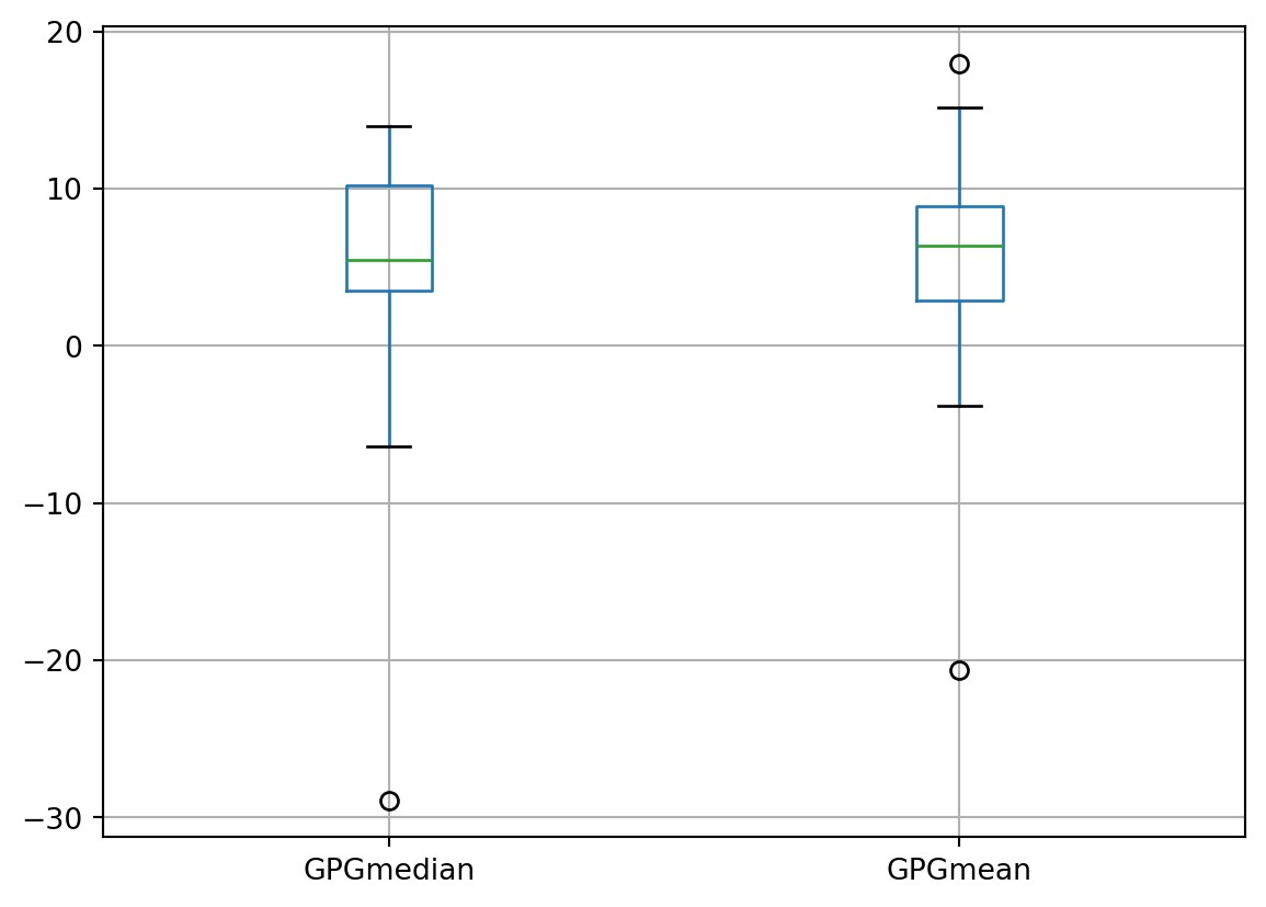
Hmmm, there are outliers. Let’s check the descriptive statistics
# Let's look at the distribution of the values in the columns
df_profession.describe()| Code | GPGmedian | GPGmean | |
|---|---|---|---|
| count | 26.000000 | 26.000000 | 25.00000 |
| mean | 47.923077 | 4.988462 | 5.70800 |
| std | 23.918065 | 8.505778 | 7.49277 |
| min | 11.000000 | -28.900000 | -20.60000 |
| 25% | 31.250000 | 3.500000 | 2.90000 |
| 50% | 46.500000 | 5.450000 | 6.40000 |
| 75% | 62.750000 | 10.200000 | 8.90000 |
| max | 92.000000 | 14.000000 | 18.00000 |
# Let's try to visualise what's going on with a histogram - what type of skew do you notice?
df_profession[['GPGmedian']].plot(kind='hist', ec='black')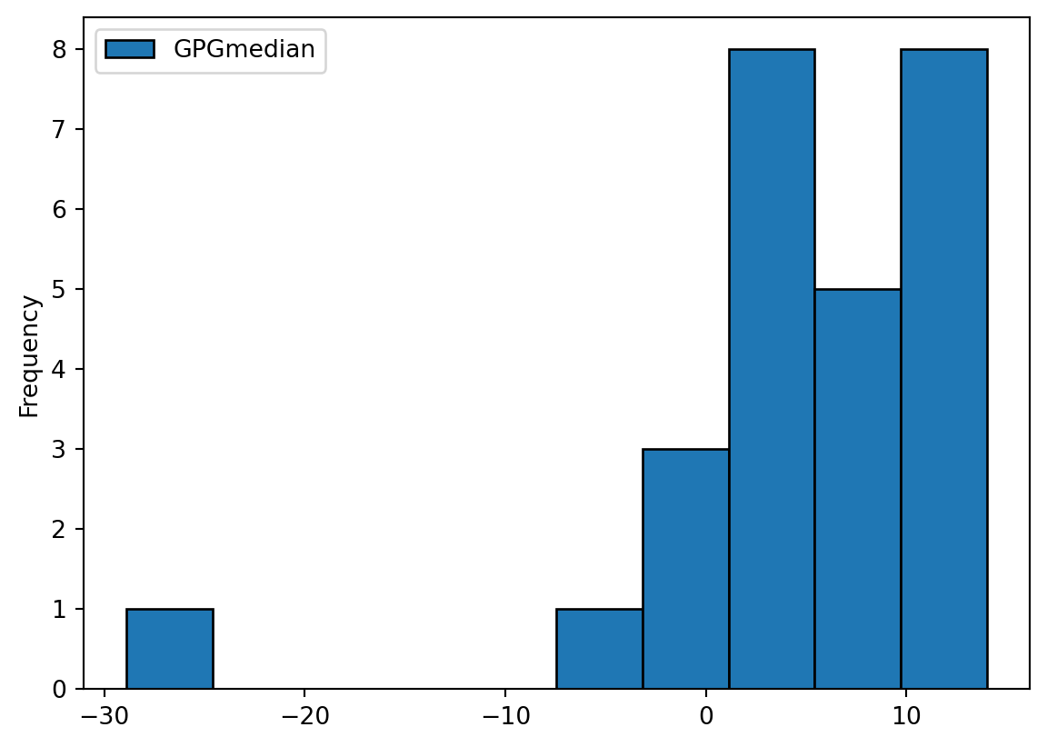
Hmmm, there appears to be a lone bin in our histogram. Which might be the profession or professions where women earn more than men?
# Is there one profession or more professions where women earn more? Let's do some investigation through visualisation.
import altair as alt
alt.Chart(df_profession).mark_bar().encode(
alt.X("GPGmedian:Q", bin=True, title='GPGmedian'),
y=alt.Y('Description:N', sort='-x', title='Professional Category'),
color='Description:N',
tooltip=['Description', 'GPGmedian']
).properties(
width=600,
height=400
)This plot shows us that Community and civil enforcement occupations, skilled agricultural and related trades, and secretarial and related occupations are the ones where women earn, on average, more than men.
If you are wondering what ‘community and civil enforcement occupations’ mean - then this ONS source says it includes police community and parking and civil enforcement officers.
Are these occupations the ones you suspected women to earn more than men (on average)?
Sidenote
The above visualisation is detailed, but it’s busy and cluttered. How about if we try doing this on df_profession_category instead?
# Is there one profession where Women earn more? Let's do some investigation.
import altair as alt
alt.Chart(df_profession_category).mark_bar().encode(
alt.X("GPGmedian:Q", bin=True),
y=alt.Y('Description:N', sort='-x'),
color='Description:N',
tooltip=['Description', 'GPGmedian']
).properties(
width=600,
height=400
)In this, we have lost some of the detail we had in the earlier visualisation, but we get to know that “Caring, leisure and other service occupations” is a ‘main category’ of occcupation where the GPG is low (but women don’t earn more than men).
Sidenote
What does this narrative tell you about women being more likely to do multiple jobs to work around their domestic responsibilities which we spoke about in the video recordings this week?
# Alternative visualisation (excluding all employees category)
# In which main professional categories is the gap narrow? Let's find out!
df_professions_sorted = df_profession_category.sort_values('GPGmedian', ascending=True)
# Let's drop the row corresponding to 'All employees' because we are more interested in looking at the differences across professional categories and sub-categories here
df_professions_sorted = df_professions_sorted[df_professions_sorted['Description'] != 'All employees']
# Let's create the bar plot
df_professions_sorted.plot.bar(x='Description', y='GPGmedian')
Let’s look at age-based differences next:
df_age.sort_values('age_group', ascending=True).plot.bar(x = 'age_group', y = 'GPGmedian')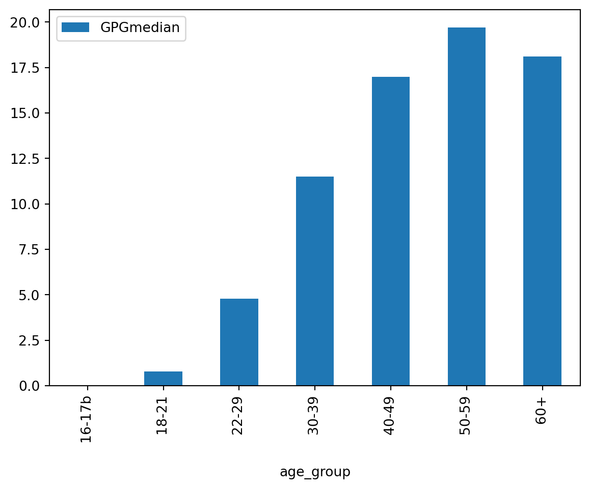
Reflection
It seems that GPG increases with age - what does this say about discussion in the lecture videos about GPG increasing for women who take time off from work for a variety of reasons compared to their male and female counterparts who do not take time out of work! What do you think might be the reasons for the minor fall in GPG at 60+?
34.4 Geography
34.4.0.1 But first:
Since moving on from our Iris and Wine datasets, the real-world datasets rarely come prepared (ready to use).
- If you download the zip file for a more recent 2023 Pay Gap ONS statistics, you will notice that they have color-coded their cells based on the certainty of estimates. On the one hand, this is very good practice - being transparent about the quality of the data. On the other hand, it tells us that we need to be careful about what insights we can draw from the data.
- If you look at the statistics for one year, you can get a glimpse of what’s happening across various categories (geography, age, profession, etc.) in terms of GPG but it’s a cross-sectional view. But you can collate a longitudinal view should you wish to. E.g., by downloading the zip folders across the desired years and collating the information for desired categories for multiple years. But remember that this will be a ‘simplified approach’ to a longitudinal view and will have limitations. Also, recollect one of the figures shown to you in the earlier lectures - it’s common to spend a lot of time at the start of your Data Science project just collating the necessary information. If you fancy, you can write a script to automate the data collation process!
- We have geography information as area codes from the ONS source, but wouldn’t it be nice if we are able to visualise GPG by Geography on a map of England (with Levelling Up agenda and all). That’s the data hunt I went on. And the ONS’ Geodata portal provides datasets from the different administrative boundaries, so I downloaded this one:Counties and Unitary Authorities (May 2023) Boundaries UK BUC. Now let’s see what visualisation we can create with it.
Takeaway
Collating data from multiple sources is a significant, valuable and legitimate part of the Data Science project journey
# Getting the geospatial polygons for England
import geopandas as gpd
import altair as alt
geo_states_england = gpd.read_file('data/Counties_and_Unitary_Authorities_May_2023_UK_BUC_-7406349609691062173.gpkg')
geo_states_england.head()| CTYUA23CD | CTYUA23NM | CTYUA23NMW | BNG_E | BNG_N | LONG | LAT | GlobalID | geometry | |
|---|---|---|---|---|---|---|---|---|---|
| 0 | E06000001 | Hartlepool | 447160 | 531474 | -1.27018 | 54.676102 | {224B1BB0-27FA-4B44-AD01-F22525CE232E} | MULTIPOLYGON (((448973.593 536745.277, 448290.... | |
| 1 | E06000002 | Middlesbrough | 451141 | 516887 | -1.21099 | 54.544701 | {8A06DF87-1F09-4A1C-9D6E-A32D40A0B159} | MULTIPOLYGON (((451894.299 521145.303, 448410.... | |
| 2 | E06000003 | Redcar and Cleveland | 464361 | 519597 | -1.00608 | 54.567501 | {4A930CE8-4656-4A98-880E-8110EE3D8501} | MULTIPOLYGON (((478232.568 518788.831, 478074.... | |
| 3 | E06000004 | Stockton-on-Tees | 444940 | 518183 | -1.30664 | 54.556900 | {304224A1-E808-4BF2-8F3E-AC43B0368BE8} | MULTIPOLYGON (((452243.536 526335.188, 451148.... | |
| 4 | E06000005 | Darlington | 428029 | 515648 | -1.56835 | 54.535301 | {F7BBD06A-7E09-4832-90D0-F6CA591D4A1D} | MULTIPOLYGON (((436388.002 522354.197, 435529.... |
print(geo_states_england.columns)Index(['CTYUA23CD', 'CTYUA23NM', 'CTYUA23NMW', 'BNG_E', 'BNG_N', 'LONG', 'LAT',
'GlobalID', 'geometry'],
dtype='object')# Let's drop the columns we don't need
geo_states_england = geo_states_england.drop(['CTYUA23NMW', 'BNG_E', 'BNG_N', 'GlobalID'], axis=1)# Let's check again
geo_states_england.head()| CTYUA23CD | CTYUA23NM | LONG | LAT | geometry | |
|---|---|---|---|---|---|
| 0 | E06000001 | Hartlepool | -1.27018 | 54.676102 | MULTIPOLYGON (((448973.593 536745.277, 448290.... |
| 1 | E06000002 | Middlesbrough | -1.21099 | 54.544701 | MULTIPOLYGON (((451894.299 521145.303, 448410.... |
| 2 | E06000003 | Redcar and Cleveland | -1.00608 | 54.567501 | MULTIPOLYGON (((478232.568 518788.831, 478074.... |
| 3 | E06000004 | Stockton-on-Tees | -1.30664 | 54.556900 | MULTIPOLYGON (((452243.536 526335.188, 451148.... |
| 4 | E06000005 | Darlington | -1.56835 | 54.535301 | MULTIPOLYGON (((436388.002 522354.197, 435529.... |
# Let's create a map of England
pre_GPG_England = alt.Chart(geo_states_england, title='Map of England').mark_geoshape().encode(
tooltip=['CTYUA23NM']
).properties(
width=500,
height=300
)
pre_GPG_EnglandWait, what’s that?! That’s not what we were expecting!
Map projections
Because the Earth is round, and maps are flat, geospatial data needs to be “projected”. There are many types of projecting geospatial data, and all of them come with some tradeoff in terms of distorting area and/or distance (in other words, none of them are perfect). You can read more here.
Now, the geospatial dataset that we are using for this notebook was downloaded from the Office for National Statistics’ Geoportal and uses a Coordinate Reference System (CRS) known as EPSG:27700 - OSGB36 / British National Grid. Regretfully, Altair works with a different CRS: WGS 84 (also known as epsg:4326), and this is creating the conflict.
We have two options: either reproject our data using geopandas, or according to Altair documentation try using the project configuration (type: 'identity', reflectY': True). It draws the geometries without applying a projection.
# Let's create a map of England
pre_GPG_England = alt.Chart(
geo_states_england, title='Map of England'
).mark_geoshape().encode(
tooltip=['CTYUA23NM']
).properties(
width=500,
height=300
).project(
type='identity',
reflectY=True
)
pre_GPG_Englanddf_geography.info()<class 'pandas.core.frame.DataFrame'>
RangeIndex: 390 entries, 0 to 389
Data columns (total 4 columns):
# Column Non-Null Count Dtype
--- ------ -------------- -----
0 Description 390 non-null object
1 Code 390 non-null object
2 GPGmedian 386 non-null float64
3 GPGmean 387 non-null float64
dtypes: float64(2), object(2)
memory usage: 12.3+ KBgeo_states_england| CTYUA23CD | CTYUA23NM | LONG | LAT | geometry | |
|---|---|---|---|---|---|
| 0 | E06000001 | Hartlepool | -1.27018 | 54.676102 | MULTIPOLYGON (((448973.593 536745.277, 448290.... |
| 1 | E06000002 | Middlesbrough | -1.21099 | 54.544701 | MULTIPOLYGON (((451894.299 521145.303, 448410.... |
| 2 | E06000003 | Redcar and Cleveland | -1.00608 | 54.567501 | MULTIPOLYGON (((478232.568 518788.831, 478074.... |
| 3 | E06000004 | Stockton-on-Tees | -1.30664 | 54.556900 | MULTIPOLYGON (((452243.536 526335.188, 451148.... |
| 4 | E06000005 | Darlington | -1.56835 | 54.535301 | MULTIPOLYGON (((436388.002 522354.197, 435529.... |
| ... | ... | ... | ... | ... | ... |
| 213 | W06000020 | Torfaen | -3.05101 | 51.698399 | MULTIPOLYGON (((333723 192653.903, 330700.402 ... |
| 214 | W06000021 | Monmouthshire | -2.90280 | 51.778301 | MULTIPOLYGON (((329597.402 229251.797, 326793.... |
| 215 | W06000022 | Newport | -2.89769 | 51.582298 | MULTIPOLYGON (((343091.833 184213.309, 342279.... |
| 216 | W06000023 | Powys | -3.43531 | 52.348598 | MULTIPOLYGON (((322891.55 333139.949, 321104.0... |
| 217 | W06000024 | Merthyr Tydfil | -3.36425 | 51.748600 | MULTIPOLYGON (((308057.304 211036.201, 306294.... |
218 rows × 5 columns
df_geography| Description | Code | GPGmedian | GPGmean | |
|---|---|---|---|---|
| 0 | Darlington UA | E06000005 | 5.4 | 13.3 |
| 1 | Hartlepool UA | E06000001 | 6.2 | 8.9 |
| 2 | Middlesbrough UA | E06000002 | 14.5 | 15.6 |
| 3 | Redcar and Cleveland UA | E06000003 | 12.8 | 12.3 |
| 4 | Stockton-on-Tees UA | E06000004 | 17.1 | 16.9 |
| ... | ... | ... | ... | ... |
| 385 | South Lanarkshire | S12000029 | 6.1 | 7.5 |
| 386 | Stirling | S12000030 | 7.4 | 21.9 |
| 387 | West Dunbartonshire | S12000039 | 17.5 | 12.8 |
| 388 | West Lothian | S12000040 | 8.3 | 9.6 |
| 389 | Northern Ireland | N92000002 | 8.1 | 9.6 |
390 rows × 4 columns
# Add the data
geo_states_england_merged = geo_states_england.merge(df_geography, left_on = 'CTYUA23CD', right_on = 'Code')# Check the merged data
geo_states_england_merged.head(10)| CTYUA23CD | CTYUA23NM | LONG | LAT | geometry | Description | Code | GPGmedian | GPGmean | |
|---|---|---|---|---|---|---|---|---|---|
| 0 | E06000001 | Hartlepool | -1.27018 | 54.676102 | MULTIPOLYGON (((448973.593 536745.277, 448290.... | Hartlepool UA | E06000001 | 6.2 | 8.9 |
| 1 | E06000002 | Middlesbrough | -1.21099 | 54.544701 | MULTIPOLYGON (((451894.299 521145.303, 448410.... | Middlesbrough UA | E06000002 | 14.5 | 15.6 |
| 2 | E06000003 | Redcar and Cleveland | -1.00608 | 54.567501 | MULTIPOLYGON (((478232.568 518788.831, 478074.... | Redcar and Cleveland UA | E06000003 | 12.8 | 12.3 |
| 3 | E06000004 | Stockton-on-Tees | -1.30664 | 54.556900 | MULTIPOLYGON (((452243.536 526335.188, 451148.... | Stockton-on-Tees UA | E06000004 | 17.1 | 16.9 |
| 4 | E06000005 | Darlington | -1.56835 | 54.535301 | MULTIPOLYGON (((436388.002 522354.197, 435529.... | Darlington UA | E06000005 | 5.4 | 13.3 |
| 5 | E06000006 | Halton | -2.68853 | 53.334202 | MULTIPOLYGON (((358131.901 385425.802, 355191.... | Halton UA | E06000006 | 3.4 | 4.6 |
| 6 | E06000007 | Warrington | -2.56167 | 53.391602 | MULTIPOLYGON (((367582.201 396058.199, 367158.... | Warrington UA | E06000007 | 12.8 | 14.6 |
| 7 | E06000008 | Blackburn with Darwen | -2.46360 | 53.700802 | MULTIPOLYGON (((372966.498 423266.501, 371465.... | Blackburn with Darwen UA | E06000008 | 22.3 | 15.3 |
| 8 | E06000009 | Blackpool | -3.02199 | 53.821602 | MULTIPOLYGON (((333572.799 437130.702, 333041.... | Blackpool UA | E06000009 | 4.4 | 3.5 |
| 9 | E06000010 | Kingston upon Hull, City of | -0.30382 | 53.769199 | MULTIPOLYGON (((515429.592 427689.472, 516047.... | Kingston upon Hull UA | E06000010 | 16.1 | 7.9 |
# Let's plot the GPG by geography now
post_GPG_England = alt.Chart(geo_states_england_merged, title='GPG by region - England').mark_geoshape().encode(
color='GPGmedian',
tooltip=['Description', 'GPGmedian']
).properties(
width=500,
height=300
).project(
type='identity',
reflectY=True
)
post_GPG_England# side by side view
GPG_England = pre_GPG_England | post_GPG_England
GPG_EnglandHow do the results in this workbook compare to related visualisations elsewhere (indicated in lecture slides too), for example, for the UK in Information is Beautiful But remember the earnings across the two might be for different years - do remember to check the metadata!