import warnings
warnings.filterwarnings('ignore')10 Lab: Seaborn
In the previous notebooks we created basic, yet fast, visualisations using matplotlib. In this one we will be using a different plotting library called Seaborn. Some consider it the ggplot of Python with excellent default setting which make your data life easier.
10.1 Preparations
As usual, we need to load any package and data needed for our work.
import numpy as np
import pandas as pd
import seaborn as sns

office_df = pd.read_csv('data/raw/office_ratings.csv', encoding='UTF-8')
And check our data:
office_df.head()| season | episode | title | imdb_rating | total_votes | air_date | |
|---|---|---|---|---|---|---|
| 0 | 1 | 1 | Pilot | 7.6 | 3706 | 2005-03-24 |
| 1 | 1 | 2 | Diversity Day | 8.3 | 3566 | 2005-03-29 |
| 2 | 1 | 3 | Health Care | 7.9 | 2983 | 2005-04-05 |
| 3 | 1 | 4 | The Alliance | 8.1 | 2886 | 2005-04-12 |
| 4 | 1 | 5 | Basketball | 8.4 | 3179 | 2005-04-19 |
We can try to replicate the same plots as in the previous notebooks.
10.2 Scatterplots
This is relatively similar to what we did in Section 8.3, but in this case we will be using seaborn’s replot() method.
sns.relplot(x='total_votes', y='imdb_rating', data=office_df)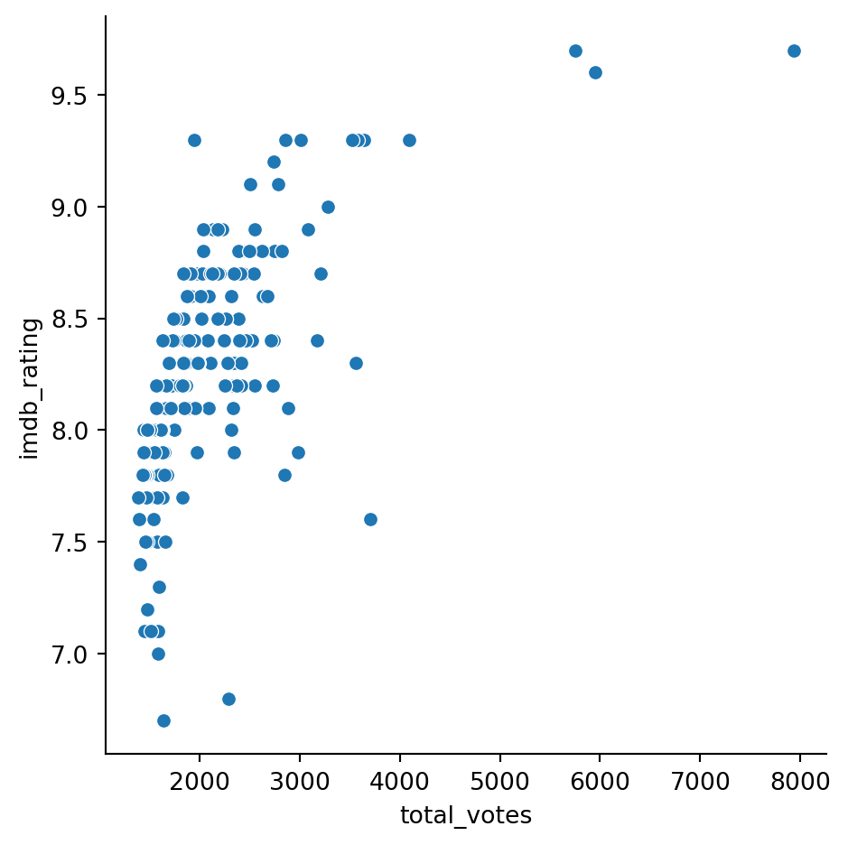
10.2.1 Dates
If we want to create a scatterplot with dates, we will need to convert them to dates, too:
office_df['air_date'] =  pd.to_datetime(office_df['air_date'], errors='ignore')

g = sns.relplot(x="air_date", y="imdb_rating", kind="scatter", data=office_df)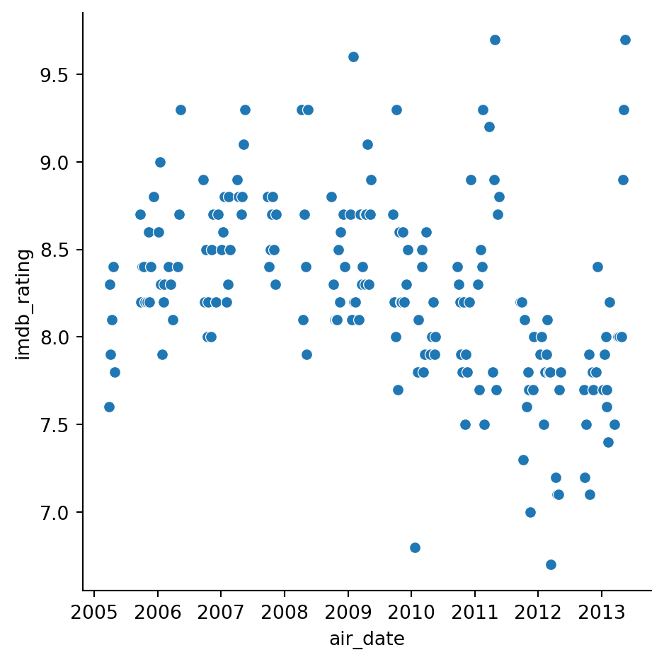
10.3 Functions
We can define our own functions. A function helps us with code we are going to run multiple times. For instance, the below function scales values between 0 and 1.
Here is a modified function from stackoverflow.
office_df.head()| season | episode | title | imdb_rating | total_votes | air_date | |
|---|---|---|---|---|---|---|
| 0 | 1 | 1 | Pilot | 7.6 | 3706 | 2005-03-24 |
| 1 | 1 | 2 | Diversity Day | 8.3 | 3566 | 2005-03-29 |
| 2 | 1 | 3 | Health Care | 7.9 | 2983 | 2005-04-05 |
| 3 | 1 | 4 | The Alliance | 8.1 | 2886 | 2005-04-12 |
| 4 | 1 | 5 | Basketball | 8.4 | 3179 | 2005-04-19 |
def normalize(df, feature_name):
    result = df.copy()

    max_value = df[feature_name].max()
    min_value = df[feature_name].min()

    result[feature_name] = (df[feature_name] - min_value) / (max_value - min_value)

    return result
Passing the dataframe and name of the column will return a dataframe with that column scaled between 0 and 1.
normalize(office_df, 'imdb_rating')| season | episode | title | imdb_rating | total_votes | air_date | |
|---|---|---|---|---|---|---|
| 0 | 1 | 1 | Pilot | 0.300000 | 3706 | 2005-03-24 |
| 1 | 1 | 2 | Diversity Day | 0.533333 | 3566 | 2005-03-29 |
| 2 | 1 | 3 | Health Care | 0.400000 | 2983 | 2005-04-05 |
| 3 | 1 | 4 | The Alliance | 0.466667 | 2886 | 2005-04-12 |
| 4 | 1 | 5 | Basketball | 0.566667 | 3179 | 2005-04-19 |
| ... | ... | ... | ... | ... | ... | ... |
| 183 | 9 | 19 | Stairmageddon | 0.433333 | 1484 | 2013-04-11 |
| 184 | 9 | 20 | Paper Airplane | 0.433333 | 1482 | 2013-04-25 |
| 185 | 9 | 21 | Livin' the Dream | 0.733333 | 2041 | 2013-05-02 |
| 186 | 9 | 22 | A.A.R.M. | 0.866667 | 2860 | 2013-05-09 |
| 187 | 9 | 23 | Finale | 1.000000 | 7934 | 2013-05-16 |
188 rows × 6 columns
Replacing the origonal dataframe. We can normalize both out votes and rating.
office_df = normalize(office_df, 'imdb_rating')office_df = normalize(office_df, 'total_votes')office_df| season | episode | title | imdb_rating | total_votes | air_date | |
|---|---|---|---|---|---|---|
| 0 | 1 | 1 | Pilot | 0.300000 | 0.353616 | 2005-03-24 |
| 1 | 1 | 2 | Diversity Day | 0.533333 | 0.332212 | 2005-03-29 |
| 2 | 1 | 3 | Health Care | 0.400000 | 0.243082 | 2005-04-05 |
| 3 | 1 | 4 | The Alliance | 0.466667 | 0.228253 | 2005-04-12 |
| 4 | 1 | 5 | Basketball | 0.566667 | 0.273047 | 2005-04-19 |
| ... | ... | ... | ... | ... | ... | ... |
| 183 | 9 | 19 | Stairmageddon | 0.433333 | 0.013912 | 2013-04-11 |
| 184 | 9 | 20 | Paper Airplane | 0.433333 | 0.013606 | 2013-04-25 |
| 185 | 9 | 21 | Livin' the Dream | 0.733333 | 0.099067 | 2013-05-02 |
| 186 | 9 | 22 | A.A.R.M. | 0.866667 | 0.224278 | 2013-05-09 |
| 187 | 9 | 23 | Finale | 1.000000 | 1.000000 | 2013-05-16 |
188 rows × 6 columns
10.3.1 Long format
Seaborn prefers a long format table. Details of melt can be found here.
office_df_long=pd.melt(office_df, id_vars=['season', 'episode', 'title', 'air_date'], value_vars=['imdb_rating', 'total_votes'])
office_df_long| season | episode | title | air_date | variable | value | |
|---|---|---|---|---|---|---|
| 0 | 1 | 1 | Pilot | 2005-03-24 | imdb_rating | 0.300000 |
| 1 | 1 | 2 | Diversity Day | 2005-03-29 | imdb_rating | 0.533333 |
| 2 | 1 | 3 | Health Care | 2005-04-05 | imdb_rating | 0.400000 |
| 3 | 1 | 4 | The Alliance | 2005-04-12 | imdb_rating | 0.466667 |
| 4 | 1 | 5 | Basketball | 2005-04-19 | imdb_rating | 0.566667 |
| ... | ... | ... | ... | ... | ... | ... |
| 371 | 9 | 19 | Stairmageddon | 2013-04-11 | total_votes | 0.013912 |
| 372 | 9 | 20 | Paper Airplane | 2013-04-25 | total_votes | 0.013606 |
| 373 | 9 | 21 | Livin' the Dream | 2013-05-02 | total_votes | 0.099067 |
| 374 | 9 | 22 | A.A.R.M. | 2013-05-09 | total_votes | 0.224278 |
| 375 | 9 | 23 | Finale | 2013-05-16 | total_votes | 1.000000 |
376 rows × 6 columns
Which we can plot in seaborn like so.
sns.relplot(x='air_date', y='value', size='variable', data=office_df_long)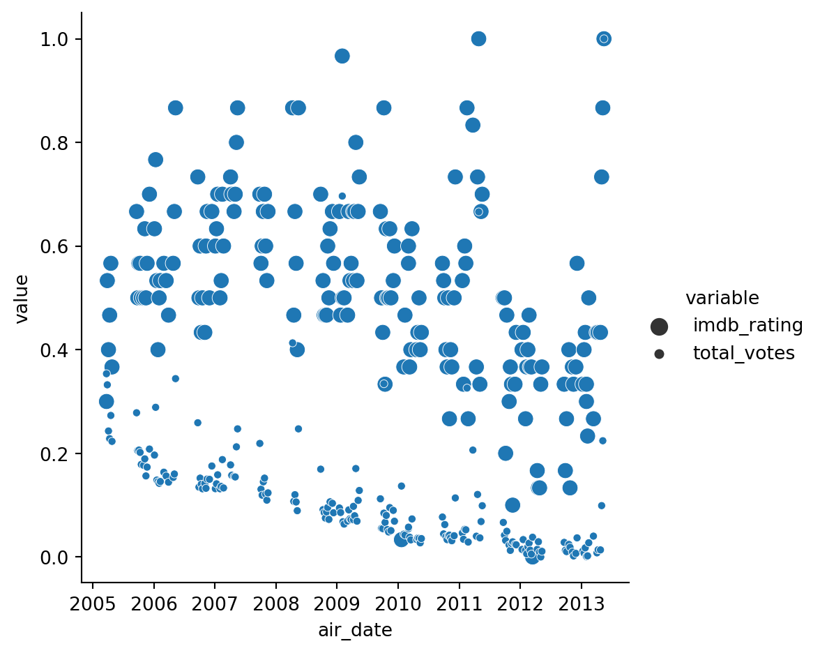
?sns.relplot