21  Lab: Working with multiple models

In this notebook, we will look at the London Borough data that we already encountered when we worked with the London Borough profiles and the Borough Cards that we utilised in the session.

You can have a look at the data through this online tool provided by GLA: https://data.london.gov.uk/london-area-profiles/

However, unlike the data that we explored during the session, this data set has several features (i.e., columns or variables), 76 of them to be precise.

What we would like to do in this notebook is to make use of a dimension reduction algorithm – Multidimensional Scaling – to help us create various different “spaces”. Each of these space will be a different way of “seeing this data” and if we adopt the language from Scott Page (2018), they will have different “attentions”.

What the following exercise will do is to walk you through the variables of this data set through a few visualisations. It will then create a few different projections and will give them some names. What we expect you to do is to create your own projections and try to interpret them.

If you want to be reminded of what MDS is, you can have a look at the slides from last week. In a super tiny nutshell, MDS tries to create a space where “real” distances in the data are preserved as much as possible while “projecting” the data elements on a lower dimensional space. For instance, the following is from the slide deck:

An MDS plot of cities.

What we see here are a few cities that would normally “exist” in our 3-dimensional world and the distances between them would normally be on this spherical coordinate system. But we create here is a 2D map and the distances between cities are preserved as much as possible. Near cities in the world are closer, and the further ones are further but not as accurate as it is in the world. The dimensions here carry no real meaning it is the distances that will “tell a story” (if there is one).

OK, let’s get on with the data now.

21.1 Data exploration and wrangling

import warnings
warnings.filterwarnings('ignore')

import pandas as pd

df = pd.read_excel('data/london-borough-profilesV3.xlsx', engine = 'openpyxl')
df.columns

Index(['Code', 'Area/INDICATOR', 'Inner/ Outer London',
       'GLA Population Estimate 2013', 'GLA Household Estimate 2013',
       'Inland Area (Hectares)', 'Population density (per hectare) 2013',
       'Average Age, 2013', 'Proportion of population aged 0-15, 2013',
       'Proportion of population of working-age, 2013',
       'Proportion of population aged 65 and over, 2013',
       '% of resident population born abroad (2013)',
       'Largest migrant population by country of birth (2013)',
       '% of largest migrant population (2013)',
       'Second largest migrant population by country of birth (2013)',
       '% of second largest migrant population (2013)',
       'Third largest migrant population by country of birth (2013)',
       '% of third largest migrant population (2013)',
       '% of population from BAME groups (2013)',
       '% people aged 3+ whose main language is not English (2011 census)',
       'Overseas nationals entering the UK (NINo), (2013/14)',
       'New migrant (NINo) rates, (2013/14)', 'Employment rate (%) (2013/14)',
       'Male employment rate (2013/14)', 'Female employment rate (2013/14)',
       'Unemployment rate (2013/14)', 'Youth Unemployment rate (2013/14)',
       'Proportion of 16-18 year olds who are NEET (%) (2013)',
       'Proportion of the working-age population who claim benefits (%) (Feb-2014)',
       '% working-age with a disability (2012)',
       'Proportion of working age people with no qualifications (%) 2013',
       'Proportion of working age people in London with degree or equivalent and above (%) 2013',
       'Gross Annual Pay, (2013)', 'Gross Annual Pay - Male (2013)',
       'Gross Annual Pay - Female (2013)',
       '% adults that volunteered in past 12 months (2010/11 to 2012/13)',
       'Number of jobs by workplace (2012)',
       '% of employment that is in public sector (2012)', 'Jobs Density, 2012',
       'Number of active businesses, 2012',
       'Two-year business survival rates 2012',
       'Crime rates per thousand population 2013/14',
       'Fires per thousand population (2013)',
       'Ambulance incidents per hundred population (2013)',
       'Median House Price, 2013',
       'Average Band D Council Tax charge (£), 2014/15',
       'New Homes (net) 2012/13', 'Homes Owned outright, (2013) %',
       'Being bought with mortgage or loan, (2013) %',
       'Rented from Local Authority or Housing Association, (2013) %',
       'Rented from Private landlord, (2013) %',
       '% of area that is Greenspace, 2005', 'Total carbon emissions (2012)',
       'Household Waste Recycling Rate, 2012/13',
       'Number of cars, (2011 Census)',
       'Number of cars per household, (2011 Census)',
       '% of adults who cycle at least once per month, 2011/12',
       'Average Public Transport Accessibility score, 2012',
       'Indices of Multiple Deprivation 2010 Rank of Average Score',
       'Income Support claimant rate (Feb-14)',
       '% children living in out-of-work families (2013)',
       'Achievement of 5 or more A*- C grades at GCSE or equivalent including English and Maths, 2012/13',
       'Rates of Children Looked After (2013)',
       '% of pupils whose first language is not English (2014)',
       'Male life expectancy, (2010-12)', 'Female life expectancy, (2010-12)',
       'Teenage conception rate (2012)',
       'Life satisfaction score 2012-13 (out of 10)',
       'Worthwhileness score 2012-13 (out of 10)',
       'Happiness score 2012-13 (out of 10)',
       'Anxiety score 2012-13 (out of 10)', 'Political control in council',
       'Proportion of seats won by Conservatives in 2014 election',
       'Proportion of seats won by Labour in 2014 election',
       'Proportion of seats won by Lib Dems in 2014 election',
       'Turnout at 2014 local elections'],
      dtype='object')

df

	Code	Area/INDICATOR	Inner/ Outer London	GLA Population Estimate 2013	GLA Household Estimate 2013	Inland Area (Hectares)	Population density (per hectare) 2013	Average Age, 2013	Proportion of population aged 0-15, 2013	Proportion of population of working-age, 2013	...	Teenage conception rate (2012)	Life satisfaction score 2012-13 (out of 10)	Worthwhileness score 2012-13 (out of 10)	Happiness score 2012-13 (out of 10)	Anxiety score 2012-13 (out of 10)	Political control in council	Proportion of seats won by Conservatives in 2014 election	Proportion of seats won by Labour in 2014 election	Proportion of seats won by Lib Dems in 2014 election	Turnout at 2014 local elections
0	E09000001	City of London	Inner London	8000	4514.371383	290.4	27.525868	41.303887	7.948036	77.541617	...	.	8.10	8.23	7.44	x	NaN	NaN	NaN	NaN	NaN
1	E09000002	Barking and Dagenham	Outer London	195600	73261.408580	3610.8	54.160527	33.228935	26.072939	63.835021	...	35.4	7.06	7.57	6.97	3.3	Lab	0.000000	100.000000	0.000000	38.16
2	E09000003	Barnet	Outer London	370000	141385.794900	8674.8	42.651374	36.896246	20.886408	65.505593	...	14.7	7.35	7.79	7.27	2.63	Cons	50.793651	42.857143	1.587302	41.1
3	E09000004	Bexley	Outer London	236500	94701.226400	6058.1	39.044243	38.883039	20.282830	63.146450	...	25.8	7.47	7.75	7.21	3.22	Cons	71.428571	23.809524	0.000000	not avail
4	E09000005	Brent	Outer London	320200	114318.553900	4323.3	74.063670	35.262694	20.462585	68.714872	...	19.6	7.23	7.32	7.09	3.33	Lab	9.523810	88.888889	1.587302	33
5	E09000006	Bromley	Outer London	317400	134012.675100	15013.5	21.137655	39.844502	19.648001	62.927051	...	24.2	7.63	7.80	7.36	3.2	Cons	85.000000	11.666667	0.000000	not avail
6	E09000007	Camden	Inner London	228400	100841.916500	2178.9	104.820985	35.842413	15.632617	73.313473	...	18.1	7.22	7.37	7.13	3.25	Lab	22.222222	74.074074	1.851852	38.69
7	E09000008	Croydon	Outer London	373100	150053.929000	8650.4	43.129707	36.570761	21.641888	65.638589	...	28.6	7.00	7.46	7.11	3.02	Lab	42.857143	57.142857	0.000000	38
8	E09000009	Ealing	Outer London	344900	126860.977600	5554.4	62.089808	35.637099	20.642035	68.216689	...	22.4	7.24	7.48	7.44	3.58	Lab	17.391304	76.811594	5.797101	41.3
9	E09000010	Enfield	Outer London	322400	124601.954700	8083.2	39.888486	36.062871	22.182556	65.114934	...	26.4	7.18	7.57	7.41	2.51	Lab	34.920635	65.079365	0.000000	37.79
10	E09000011	Greenwich	Outer London	262800	104999.593900	4733.4	55.516088	34.737054	21.754144	67.650982	...	34.7	7.16	7.49	7.05	3.68	Lab	15.686275	84.313725	0.000000	37.25
11	E09000012	Hackney	Inner London	256600	106655.687500	1904.9	134.717347	32.624060	20.513252	72.376652	...	28.8	7.07	7.42	7.02	3.61	Lab	7.017544	87.719298	5.263158	42.89
12	E09000013	Hammersmith and Fulham	Inner London	181000	79688.691790	1639.7	110.384364	34.933408	16.764645	73.768103	...	25.6	7.23	7.60	6.94	3.15	Lab	43.478261	56.521739	0.000000	38
13	E09000014	Haringey	Inner London	263100	105459.284200	2959.8	88.883425	34.384912	19.877305	71.199466	...	33.1	7.20	7.44	7.13	3.07	Lab	0.000000	84.210526	15.789474	38.1
14	E09000015	Harrow	Outer London	245900	86968.599850	5046.3	48.722544	37.695216	20.110244	65.413384	...	14.2	7.34	7.53	7.35	3.17	Lab	41.269841	53.968254	1.587302	41
15	E09000016	Havering	Outer London	242600	99202.437800	11235.0	21.589910	40.296140	18.781558	62.788014	...	26.4	7.40	7.65	7.24	3.17	No Overall Control	40.740741	1.851852	0.000000	43
16	E09000017	Hillingdon	Outer London	287500	104650.805600	11570.1	24.851919	36.171629	20.911751	66.121424	...	27.7	7.35	7.63	7.34	3.34	Cons	64.615385	35.384615	0.000000	35.76
17	E09000018	Hounslow	Outer London	264300	98840.744350	5597.8	47.209459	35.263763	20.616902	68.542073	...	30.4	7.30	7.60	7.29	3.51	Lab	18.333333	81.666667	0.000000	36.8
18	E09000019	Islington	Inner London	215900	97616.282240	1485.7	145.324910	34.419467	15.863559	75.457376	...	30.1	7.08	7.22	6.85	3.74	Lab	0.000000	97.916667	0.000000	38.4
19	E09000020	Kensington and Chelsea	Inner London	155700	77210.897790	1212.4	128.427401	38.308554	15.908516	70.878237	...	17.7	7.68	7.92	7.51	3.06	Cons	74.000000	24.000000	2.000000	not avail
20	E09000021	Kingston upon Thames	Outer London	166400	65782.630740	3726.1	44.660475	36.885957	18.994951	67.980436	...	20	7.29	7.45	7.18	3.23	Cons	58.333333	4.166667	37.500000	not avail
21	E09000022	Lambeth	Inner London	313800	134512.450200	2681.0	117.055632	33.862641	17.899970	74.455090	...	33.2	7.09	7.40	6.97	3.69	Lab	4.761905	93.650794	0.000000	32
22	E09000023	Lewisham	Inner London	286000	120439.358900	3514.9	81.366697	34.540168	20.620499	69.996836	...	42	7.23	7.71	7.13	3.35	Lab	0.000000	98.148148	0.000000	37.2
23	E09000024	Merton	Outer London	205400	81047.637240	3762.5	54.603478	36.262610	20.203379	67.896608	...	25.5	7.18	7.54	7.13	3.59	Lab	33.333333	60.000000	1.666667	41
24	E09000025	Newham	Inner London	323400	107793.332200	3619.8	89.338992	31.423439	22.508503	70.809763	...	24.1	7.22	7.51	7.32	3.36	Lab	0.000000	100.000000	0.000000	40.62
25	E09000026	Redbridge	Outer London	289900	103053.713300	5641.9	51.374341	35.531757	22.684198	65.238253	...	16.2	7.28	7.44	7.34	3.12	Lab	39.682540	55.555556	4.761905	39.7
26	E09000027	Richmond upon Thames	Outer London	191300	81353.161690	5740.7	33.331460	38.290205	20.202975	65.548776	...	19.9	7.42	7.69	7.33	3.56	Cons	72.222222	0.000000	27.777778	46.3
27	E09000028	Southwark	Inner London	298400	124613.892000	2886.2	103.403127	33.754401	18.507644	73.722633	...	31.8	7.27	7.68	7.20	3.28	Lab	3.174603	76.190476	20.634921	not avail
28	E09000029	Sutton	Outer London	196400	80748.477060	4384.7	44.802887	38.310437	20.151661	64.951011	...	25.8	7.25	7.57	7.13	3.34	Lib Dem	16.666667	0.000000	83.333333	42.2
29	E09000030	Tower Hamlets	Inner London	271100	109280.540100	1978.1	137.067542	31.064282	19.602621	74.531880	...	24.3	7.28	7.56	7.32	2.93	Tower Hamlets First	15.555556	44.444444	0.000000	not avail
30	E09000031	Waltham Forest	Outer London	267700	100524.458900	3880.8	68.970286	34.502988	21.784829	68.105760	...	29.9	7.24	7.72	7.26	2.99	Lab	26.666667	73.333333	0.000000	not avail
31	E09000032	Wandsworth	Inner London	311800	131562.012900	3426.4	91.009107	34.414955	17.342442	73.693151	...	25.5	7.23	7.55	7.28	3.55	Cons	68.333333	31.666667	0.000000	not avail
32	E09000033	Westminster	Inner London	226600	108550.111900	2148.7	105.457732	36.729055	14.781940	73.924420	...	21.2	7.09	7.44	7.09	3.58	Cons	73.333333	26.666667	0.000000	not avail

33 rows × 76 columns

Lots of different features. We also have really odd NaN values such as x and not avail. We can try and get rid of this.

def isnumber(x):
    try:
        float(x)
        return True
    except:
        if (len(x) > 1) & ("not avail" not in x):
            return True
        else:
            return False

# apply isnumber function to every element
df = df[df.applymap(isnumber)]
df.head()

	Code	Area/INDICATOR	Inner/ Outer London	GLA Population Estimate 2013	GLA Household Estimate 2013	Inland Area (Hectares)	Population density (per hectare) 2013	Average Age, 2013	Proportion of population aged 0-15, 2013	Proportion of population of working-age, 2013	...	Teenage conception rate (2012)	Life satisfaction score 2012-13 (out of 10)	Worthwhileness score 2012-13 (out of 10)	Happiness score 2012-13 (out of 10)	Anxiety score 2012-13 (out of 10)	Political control in council	Proportion of seats won by Conservatives in 2014 election	Proportion of seats won by Labour in 2014 election	Proportion of seats won by Lib Dems in 2014 election	Turnout at 2014 local elections
0	E09000001	City of London	Inner London	8000	4514.371383	290.4	27.525868	41.303887	7.948036	77.541617	...	NaN	8.10	8.23	7.44	NaN	NaN	NaN	NaN	NaN	NaN
1	E09000002	Barking and Dagenham	Outer London	195600	73261.408580	3610.8	54.160527	33.228935	26.072939	63.835021	...	35.4	7.06	7.57	6.97	3.3	Lab	0.000000	100.000000	0.000000	38.16
2	E09000003	Barnet	Outer London	370000	141385.794900	8674.8	42.651374	36.896246	20.886408	65.505593	...	14.7	7.35	7.79	7.27	2.63	Cons	50.793651	42.857143	1.587302	41.1
3	E09000004	Bexley	Outer London	236500	94701.226400	6058.1	39.044243	38.883039	20.282830	63.146450	...	25.8	7.47	7.75	7.21	3.22	Cons	71.428571	23.809524	0.000000	NaN
4	E09000005	Brent	Outer London	320200	114318.553900	4323.3	74.063670	35.262694	20.462585	68.714872	...	19.6	7.23	7.32	7.09	3.33	Lab	9.523810	88.888889	1.587302	33

5 rows × 76 columns

That looks much cleaner. The missing values are all NaN now. This will help us fill them in and/or address them in some way.

# get only numeric columns
numericColumns = df._get_numeric_data()
numericColumns.head()

	GLA Population Estimate 2013	GLA Household Estimate 2013	Inland Area (Hectares)	Population density (per hectare) 2013	Average Age, 2013	Proportion of population aged 0-15, 2013	Proportion of population of working-age, 2013	Proportion of population aged 65 and over, 2013	% of population from BAME groups (2013)	% people aged 3+ whose main language is not English (2011 census)	...	Average Public Transport Accessibility score, 2012	Indices of Multiple Deprivation 2010 Rank of Average Score	Income Support claimant rate (Feb-14)	Rates of Children Looked After (2013)	Life satisfaction score 2012-13 (out of 10)	Worthwhileness score 2012-13 (out of 10)	Happiness score 2012-13 (out of 10)	Proportion of seats won by Conservatives in 2014 election	Proportion of seats won by Labour in 2014 election	Proportion of seats won by Lib Dems in 2014 election
0	8000	4514.371383	290.4	27.525868	41.303887	7.948036	77.541617	14.510348	22.557238	17.138103	...	7.631205	262	0.527983	98	8.10	8.23	7.44	NaN	NaN	NaN
1	195600	73261.408580	3610.8	54.160527	33.228935	26.072939	63.835021	10.092040	45.712357	18.724201	...	2.994817	22	4.041773	76	7.06	7.57	6.97	0.000000	100.000000	0.000000
2	370000	141385.794900	8674.8	42.651374	36.896246	20.886408	65.505593	13.607999	37.148811	23.405037	...	2.994527	176	1.736905	37	7.35	7.79	7.27	50.793651	42.857143	1.587302
3	236500	94701.226400	6058.1	39.044243	38.883039	20.282830	63.146450	16.570720	19.620095	6.031289	...	2.513007	174	2.236355	47	7.47	7.75	7.21	71.428571	23.809524	0.000000
4	320200	114318.553900	4323.3	74.063670	35.262694	20.462585	68.714872	10.822543	64.948141	37.151120	...	3.702753	35	2.256102	49	7.23	7.32	7.09	9.523810	88.888889	1.587302

5 rows × 41 columns

# the above piece of code is throwing a lot of features out for not being a numeric column. The resulting frame has 41 features, however, we would expect more.
# upon a bit of debugging, we found out that --  df._get_numeric_data() -- a Pandas function -- has a minor bug in inferring which columns are numeric when the first value of a column is a missing value, i.e., 'NaN' value. 
# This meant that some columns that are numeric were removed from the dataset even though they are numeric. 


# this next piece of code is addressing that now and also fills in the missing values with the mean() value of a column

for column_name, column in df.items():
    try:
        df[column_name] = df[column_name].fillna(df[column_name].mean())
    except:
        print("Column:", column_name, " is not a numeric column")

Column: Code  is not a numeric column
Column: Area/INDICATOR  is not a numeric column
Column: Inner/ Outer London  is not a numeric column
Column: Largest migrant population by country of birth (2013)  is not a numeric column
Column: Second largest migrant population by country of birth (2013)  is not a numeric column
Column: Third largest migrant population by country of birth (2013)  is not a numeric column
Column: Political control in council  is not a numeric column

# get only numeric columns
numericColumns = df._get_numeric_data()
numericColumns.head()

	GLA Population Estimate 2013	GLA Household Estimate 2013	Inland Area (Hectares)	Population density (per hectare) 2013	Average Age, 2013	Proportion of population aged 0-15, 2013	Proportion of population of working-age, 2013	Proportion of population aged 65 and over, 2013	% of resident population born abroad (2013)	% of largest migrant population (2013)	...	Female life expectancy, (2010-12)	Teenage conception rate (2012)	Life satisfaction score 2012-13 (out of 10)	Worthwhileness score 2012-13 (out of 10)	Happiness score 2012-13 (out of 10)	Anxiety score 2012-13 (out of 10)	Proportion of seats won by Conservatives in 2014 election	Proportion of seats won by Labour in 2014 election	Proportion of seats won by Lib Dems in 2014 election	Turnout at 2014 local elections
0	8000	4514.371383	290.4	27.525868	41.303887	7.948036	77.541617	14.510348	35.883871	5.194357	...	83.809375	25.728125	8.10	8.23	7.44	3.284688	32.854444	56.615819	6.598065	39.054783
1	195600	73261.408580	3610.8	54.160527	33.228935	26.072939	63.835021	10.092040	35.789474	5.814975	...	82.000000	35.400000	7.06	7.57	6.97	3.300000	0.000000	100.000000	0.000000	38.160000
2	370000	141385.794900	8674.8	42.651374	36.896246	20.886408	65.505593	13.607999	35.854342	2.234626	...	84.500000	14.700000	7.35	7.79	7.27	2.630000	50.793651	42.857143	1.587302	41.100000
3	236500	94701.226400	6058.1	39.044243	38.883039	20.282830	63.146450	16.570720	16.450216	2.169910	...	84.400000	25.800000	7.47	7.75	7.21	3.220000	71.428571	23.809524	0.000000	39.054783
4	320200	114318.553900	4323.3	74.063670	35.262694	20.462585	68.714872	10.822543	53.307393	10.717273	...	84.500000	19.600000	7.23	7.32	7.09	3.330000	9.523810	88.888889	1.587302	33.000000

5 rows × 69 columns

Now we have 69 columns. Looks much better than 41, we can move on!

::: callout-warning

Reflect here whether the mean() replacements for missing values taht we did above is sensible and/or would work for each and every column here. You might need more sophisticated methods for filling in some of the missing values, e.g., using a model-based approach to ‘predict’ a value.

from sklearn.metrics import euclidean_distances

# keep place names and store them in a variable
placeNames = df["Area/INDICATOR"]

# if we hadn't done it, we could have filled in the missing values also here.
# numericColumns = numericColumns.fillna(numericColumns.mean())

# let's centralize the data
numericColumns -= numericColumns.mean()

Check to make sure everything looks ok.

numericColumns.head()

	GLA Population Estimate 2013	GLA Household Estimate 2013	Inland Area (Hectares)	Population density (per hectare) 2013	Average Age, 2013	Proportion of population aged 0-15, 2013	Proportion of population of working-age, 2013	Proportion of population aged 65 and over, 2013	% of resident population born abroad (2013)	% of largest migrant population (2013)	...	Female life expectancy, (2010-12)	Teenage conception rate (2012)	Life satisfaction score 2012-13 (out of 10)	Worthwhileness score 2012-13 (out of 10)	Happiness score 2012-13 (out of 10)	Anxiety score 2012-13 (out of 10)	Proportion of seats won by Conservatives in 2014 election	Proportion of seats won by Labour in 2014 election	Proportion of seats won by Lib Dems in 2014 election	Turnout at 2014 local elections
0	-247760.606061	-97761.616805	-4473.681818	-43.279630	5.426932	-11.500067	8.480871	3.019196	0.000000	0.000000	...	-1.421085e-14	-3.552714e-15	0.816364	0.651212	0.23303	8.881784e-16	0.000000	0.000000	-8.881784e-16	7.105427e-15
1	-60160.606061	-29014.579608	-1153.281818	-16.644971	-2.648021	6.624837	-5.225725	-1.399112	-0.094397	0.620617	...	-1.809375e+00	9.671875e+00	-0.223636	-0.008788	-0.23697	1.531250e-02	-32.854444	43.384181	-6.598065e+00	-8.947826e-01
2	114239.393939	39109.806712	3910.718182	-28.154125	1.019290	1.438305	-3.555153	2.116847	-0.029529	-2.959732	...	6.906250e-01	-1.102813e+01	0.066364	0.211212	0.06303	-6.546875e-01	17.939207	-13.758676	-5.010764e+00	2.045217e+00
3	-19260.606061	-7574.761788	1294.018182	-31.761255	3.006083	0.834727	-5.914296	5.079569	-19.433655	-3.024448	...	5.906250e-01	7.187500e-02	0.186364	0.171212	0.00303	-6.468750e-02	38.574127	-32.806295	-6.598065e+00	7.105427e-15
4	64439.393939	12042.565712	-440.781818	3.258171	-0.614262	1.014482	-0.345874	-0.668608	17.423522	5.522915	...	6.906250e-01	-6.128125e+00	-0.053636	-0.258788	-0.11697	4.531250e-02	-23.330634	32.273070	-5.010764e+00	-6.054783e+00

5 rows × 69 columns

We can plot out our many dimension space by uncommenting the code below (also note down how long does this take).

#import seaborn as sns
#sns_plot = sns.pairplot(numericColumns)
#sns_plot.savefig("figs/output.png")

Given that this takes quite a while (around 10 minutes), this is the image that would result from uncommenting and running the code above.

Dimension reduction will help us here!

21.2 Multidimensional scaling

We could apply various different types of dimension reduction here. We are specifically going to capture the dissimilarity in the data using multidimensional scaling. We will need a distance matrix to start here.

from sklearn import manifold

# Here, we compute the euclidean distances between the columns by passing the same data twice
# the resulting data matrix will now have the pairwise distances between the boroughs.
# CAUTION: note that we are now building a distance matrix in a high-dimensional data space
# remember the Curse of Dimensionality -- we need to be cautious with the distance values
distMatrix = euclidean_distances(numericColumns, numericColumns)

# for instance, typing distMatrix.shape on the console gives:
# Out[115]: (38, 38) # i.e., the number of rows

# first we generate an MDS object and extract the projections
mds = manifold.MDS(n_components = 2, max_iter=3000, n_init=1, dissimilarity="precomputed", normalized_stress=False)
Y = mds.fit_transform(distMatrix)

To interpret what is happening, let us plot the boroughs on the projected two dimensional space.

from matplotlib import pyplot as plt

fig, ax = plt.subplots()
fig.set_size_inches(15, 15)
plt.suptitle('MDS on only London boroughs')
ax.scatter(Y[:, 0], Y[:, 1], c="#D06B36", s = 100, alpha = 0.8, linewidth=0)

for i, txt in enumerate(placeNames):
    ax.annotate(txt, (Y[:, 0][i],Y[:, 1][i]))

Here, we are projecting all the numeric variables, so it is difficult to get a sense of what these components represent and how to interpret the visualisation. We may want to project only a subset of features.

Feature selection

Feature selection is not straightforward and it is always a decision made by us informed by something (i.e. measures, literature –refer to the slides from last week). Below we will be embedding (machine learners’ word for projection) two different sets of features for you to compare.

21.2.1 Feature selection: Happiness

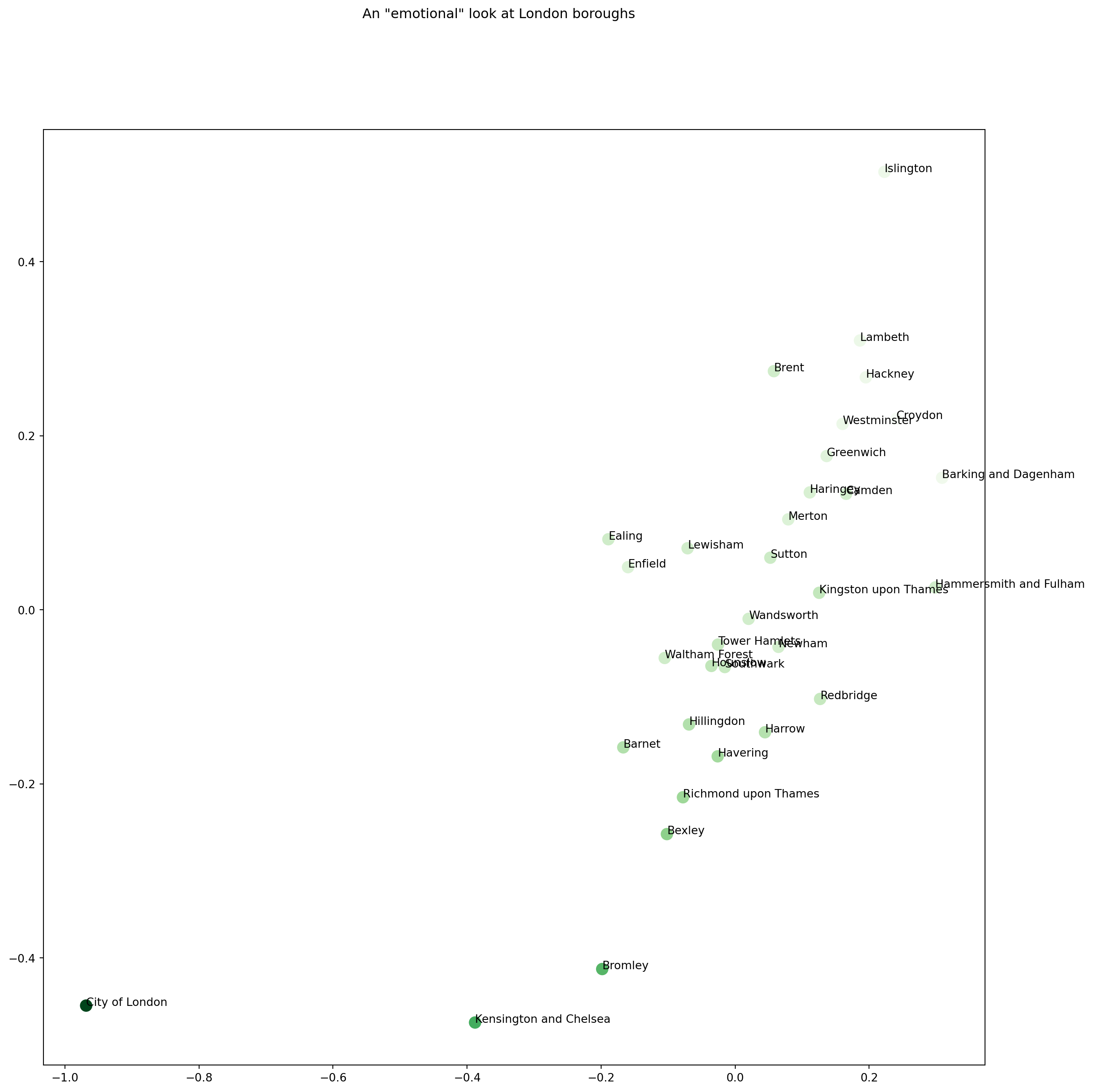
In the example below, we are selecting happiness metrics. Pulling these out of our data and carrying out more multidimensional scaling can help us see how the boroughs differ in happiness.

Note

The decision of selecting the features Life satisfaction score 2012-13 (out of 10), Worthwhileness score 2012-13 (out of 10) and Happiness score 2012-13 (out of 10) is not based on any numerical decision, but it is based on the semantics of the variables. In other words, these three variables provide different perspectives to describe how happy people are in the different neighbourhoods.

# get the data columns relating to emotions and feelings
dataOnEmotions = numericColumns[["Life satisfaction score 2012-13 (out of 10)", "Worthwhileness score 2012-13 (out of 10)","Happiness score 2012-13 (out of 10)"]]

# a new distance matrix to represent "emotional distance"s
distMatrix2 = euclidean_distances(dataOnEmotions, dataOnEmotions)

# compute a new "embedding" (machine learners' word for projection)
Y2 = mds.fit_transform(distMatrix2)

# let's look at the results
fig, ax = plt.subplots()
fig.set_size_inches(15, 15)
plt.suptitle('An \"emotional\" look at London boroughs')
ax.scatter(Y2[:, 0], Y2[:, 1], c="#D06B36", s = 100, alpha = 0.8, linewidth=0)

for i, txt in enumerate(placeNames):
    ax.annotate(txt, (Y2[:, 0][i],Y2[:, 1][i]))

The location of the different boroughs on the 2 dimensional multidimensional scaling space from the happiness metrics is

results_fixed = Y2.copy()
print(results_fixed)

[[-0.96842689 -0.45475988]
 [ 0.30884742  0.15179769]
 [-0.16691283 -0.15803682]
 [-0.10177693 -0.25768786]
 [ 0.05785895  0.27427657]
 [-0.19834493 -0.41277366]
 [ 0.16569283  0.13333937]
 [ 0.24063752  0.21942675]
 [-0.18913393  0.08113099]
 [-0.1598099   0.04904532]
 [ 0.13658172  0.1767544 ]
 [ 0.19499445  0.26719731]
 [ 0.29875164  0.0257805 ]
 [ 0.11141595  0.13492429]
 [ 0.04459044 -0.14066626]
 [-0.02600529 -0.16833037]
 [-0.06882347 -0.1317033 ]
 [-0.03540934 -0.0644621 ]
 [ 0.22277681  0.50326906]
 [-0.38808697 -0.47422441]
 [ 0.1254132   0.01958298]
 [ 0.18626664  0.30951748]
 [-0.07094936  0.07075891]
 [ 0.07928372  0.10396892]
 [ 0.06468159 -0.04256096]
 [ 0.12678319 -0.10240873]
 [-0.07785182 -0.21537067]
 [-0.0153771  -0.065743  ]
 [ 0.05253965  0.05991075]
 [-0.02558256 -0.03995683]
 [-0.10504585 -0.05529746]
 [ 0.0201215  -0.01035603]
 [ 0.16029994  0.21365705]]

print(results_fixed.shape)

(33, 2)

We may want to look at if the general happiness rating captures the position of the boroughs. To do this, we need to assign colours based on the binned happiness score.

import numpy as np

colorMappingValuesHappiness = np.asarray(dataOnEmotions[["Life satisfaction score 2012-13 (out of 10)"]]).flatten()
colorMappingValuesHappiness.shape

(33,)

colorMappingValuesHappiness
#c = colorMappingValuesCrime, cmap = plt.cm.Greens

array([ 0.81636364, -0.22363636,  0.06636364,  0.18636364, -0.05363636,
        0.34636364, -0.06363636, -0.28363636, -0.04363636, -0.10363636,
       -0.12363636, -0.21363636, -0.05363636, -0.08363636,  0.05636364,
        0.11636364,  0.06636364,  0.01636364, -0.20363636,  0.39636364,
        0.00636364, -0.19363636, -0.05363636, -0.10363636, -0.06363636,
       -0.00363636,  0.13636364, -0.01363636, -0.03363636, -0.00363636,
       -0.04363636, -0.05363636, -0.19363636])

Finally, we can plot this. What can you see?

# let's look at the results
fig, ax = plt.subplots()
fig.set_size_inches(15, 15)
plt.suptitle('An \"emotional\" look at London boroughs')
#ax.scatter(results_fixed[:, 0], results_fixed[:, 1], c = colorMappingValuesHappiness, cmap='viridis')
plt.scatter(results_fixed[:, 0], results_fixed[:, 1], c = colorMappingValuesHappiness, s = 100, cmap=plt.cm.Greens)

for i, txt in enumerate(placeNames):
    ax.annotate(txt, (results_fixed[:, 0][i],results_fixed[:, 1][i]))

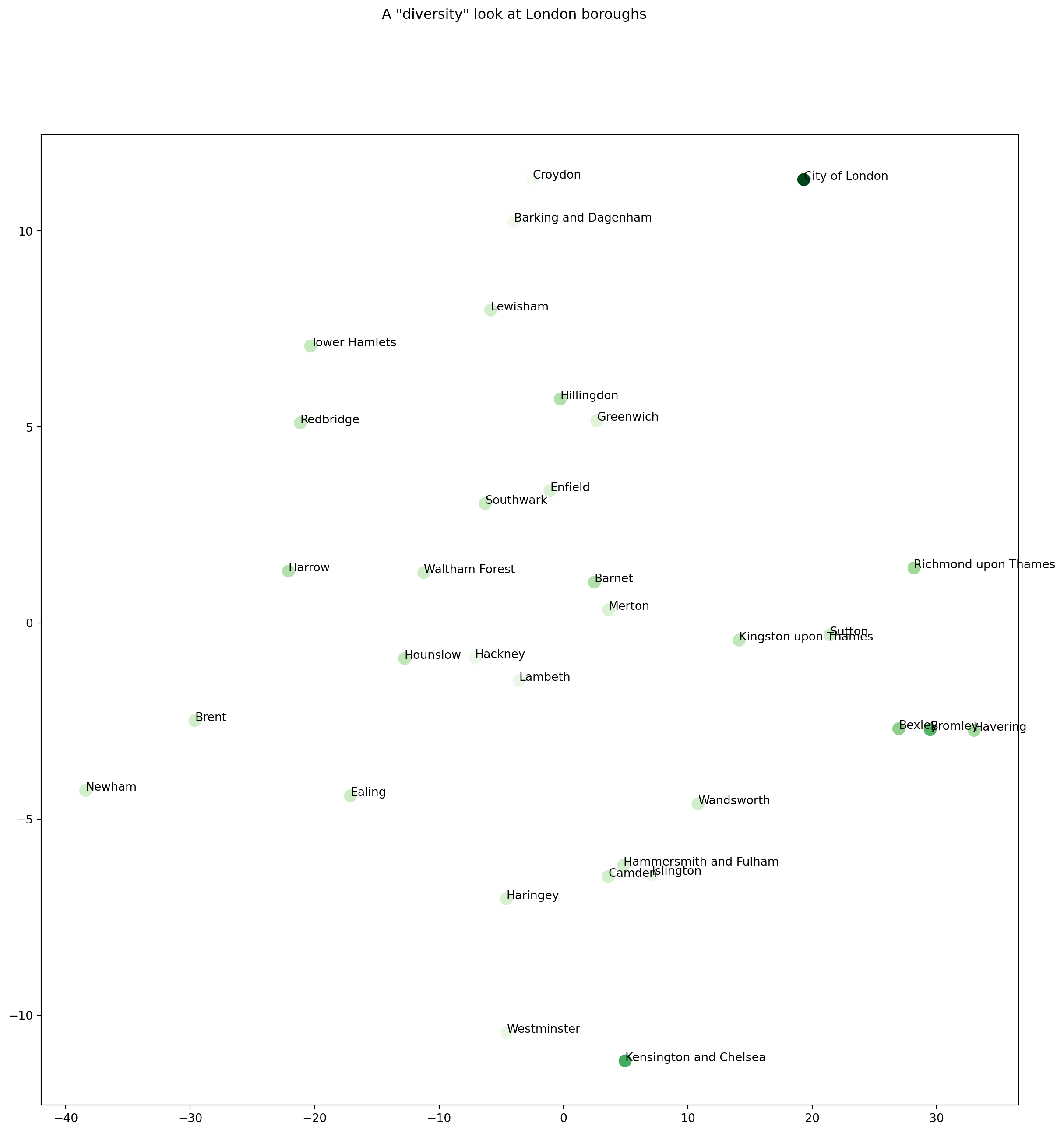
21.2.2 Feature selection: diversity

Similarly, we are now selecting features based on diveristy.

# get the data columns relating to indicators that we think are related to "diversity" in one way or the other
dataOnDiversity = numericColumns[["Proportion of population aged 0-15, 2013", "Proportion of population of working-age, 2013", "Proportion of population aged 65 and over, 2013", "% of population from BAME groups (2013)", "% people aged 3+ whose main language is not English (2011 census)"]]

# a new distance matrix to represent distances in "diversity"
distMatrix3 = euclidean_distances(dataOnDiversity, dataOnDiversity)

mds = manifold.MDS(n_components = 2, max_iter=3000, n_init=1, dissimilarity="precomputed", normalized_stress = False)
Y = mds.fit_transform(distMatrix3)

# Visualising the data.
fig, ax = plt.subplots()
fig.set_size_inches(15, 15)
plt.suptitle('A \"diversity\" look at London boroughs')
ax.scatter(Y[:, 0], Y[:, 1], s = 100, c = colorMappingValuesHappiness, cmap=plt.cm.Greens)

for i, txt in enumerate(placeNames):
    ax.annotate(txt, (Y[:, 0][i],Y[:, 1][i]))

21.3 It is now your turn!

It is your turn now

First task:

This looks very different to the one above on “emotion” related variables. Our job now is to relate these two projections to one another. Do you see similarities? Do you see clusters of boroughs? Can you reflect on how you can relate and combine these two maps conceptually?

Second task:

Can you think of and then generate other maps that you can produce with this data? Have a look at the variables once again and try to produce new “perspectives” to the data and see what they have to say.

Also think of visualisations to help you here, can you colour them with a different variable? What would that change?

Page, Scott E. 2018. “Why ‘Many-Model Thinkers’ Make Better Decisions.” Harvard Business Review, November. https://hbr.org/2018/11/why-many-model-thinkers-make-better-decisions.